Abiotic and biogeochemical signals derived from the seasonal cycles of tropospheric nitrous oxide

(1)

ACPD

10, 25803–25839, 2010

Abiotic and biogeochemical

signals

C. D. Nevison et al.

Title Page

Abstract Introduction

Conclusions References

Tables Figures

◭ ◮

Back Close

Full Screen / Esc

Printer-friendly Version Interactive Discussion

Discussion

P

a

per

|

Dis

cussion

P

a

per

|

Discussion

P

a

per

|

Discussio

n

P

a

per

|

Atmos. Chem. Phys. Discuss., 10, 25803–25839, 2010 www.atmos-chem-phys-discuss.net/10/25803/2010/ doi:10.5194/acpd-10-25803-2010

Atmospheric Chemistry and Physics Discussions

This discussion paper is/has been under review for the journal Atmospheric Chemistry and Physics (ACP). Please refer to the corresponding final paper in ACP if available.

Abiotic and biogeochemical signals

derived from the seasonal cycles of

tropospheric nitrous oxide

C. D. Nevison1, E. Dlugokencky2, G. Dutton2,3, J. W. Elkins2, P. Fraser4, B. Hall2, P. B. Krummel4, R. L. Langenfelds4, R. G. Prinn5, L. P. Steele4, and R. F. Weiss6

1

University of Colorado/INSTAAR, Boulder, Colorado, USA

2

NOAA Earth System Research Laboratory, Global Monitoring Division, Boulder, CO 80305, USA

3

University of Colorado, Cooperative Institute for Research in Environmental Sciences, Boulder, CO, USA

4

Centre for Australian Weather and Climate Research/CSIRO Marine and Atmospheric Research, Aspendale, Victoria, 3195 Australia

5

Center for Global Change Science, Department of Earth, Atmospheric, and Planetary Science, Massachusetts Institute of Technology, Cambridge, MA 02139-4307, USA

6

(2)

ACPD

10, 25803–25839, 2010

signals

Title Page

Tables Figures

◭ ◮

Back Close

Full Screen / Esc

Discussion

P

a

per

|

Dis

cussion

P

a

per

|

Discussion

P

a

per

|

Discussio

n

P

a

per

Received: 17 September 2010 – Accepted: 15 October 2010 – Published: 3 November 2010 Correspondence to: C. D. Nevison (nevison@colorado.edu)

(3)

ACPD

10, 25803–25839, 2010

signals

Title Page

Tables Figures

◭ ◮

Back Close

Full Screen / Esc

Discussion

P

a

per

|

Dis

cussion

P

a

per

|

Discussion

P

a

per

|

Discussio

n

P

a

per

|

Abstract

Seasonal cycles in the mixing ratios of tropospheric nitrous oxide (N2O) are derived

by detrending long-term measurements made at sites across four global surface mon-itoring networks. These cycles are examined for physical and biogeochemical signals. The detrended monthly data display large interannual variability, which at some sites

5

challenges the concept of a “mean” seasonal cycle. The interannual variability in the seasonal cycle is not always correlated among networks that share common sites. In the Northern Hemisphere, correlations between detrended N2O seasonal minima and

polar winter lower stratospheric temperature provide compelling evidence for a strato-spheric influence, which varies in strength from year to year and can explain much of

10

the interannual variability in the surface seasonal cycle. Even at sites where a strong, competing, regional N2O source exists, such as from coastal upwelling at Trinidad

Head, California, the stratospheric influence must be understood in order to interpret the biogeochemical signal in monthly mean data. In the Southern Hemisphere, de-trended surface N2O monthly means are correlated with polar lower stratospheric

tem-15

perature in months preceding the N2O minimum, suggesting a coherent stratospheric

influence in that hemisphere as well. A decomposition of the N₂O seasonal cycle in the extratropical Southern Hemisphere suggests that ventilation of deep ocean water (microbially enriched in N2O) and the stratospheric influx make similar contributions in

phasing, and may be di_fficult to disentangle. In addition, there is a thermal signal in

20

N2O due to seasonal ingassing and outgassing of cooling and warming surface waters

that is out of phase and thus competes with the stratospheric and ventilation signals. All the seasonal signals discussed above are subtle and are generally better quantified in high-frequency in situ data than in data from weekly flask samples, especially in the Northern Hemisphere. The importance of abiotic influences (thermal, stratospheric

in-25

flux, and tropospheric transport) on N₂O seasonal cycles suggests that, at many sites, surface N2O mixing ratio data by themselves are unlikely to provide information about

(4)

ACPD

10, 25803–25839, 2010

signals

Title Page

Tables Figures

◭ ◮

Back Close

Full Screen / Esc

Discussion

P

a

per

|

Dis

cussion

P

a

per

|

Discussion

P

a

per

|

Discussio

n

P

a

per

powerful if combined with complementary data such as CFC-12 mixing ratios or N₂O isotopes.

1 Introduction

Nitrous oxide (N₂O) is an important greenhouse gase with a global warming potential about 300 times that of CO2(Forster et al., 2007). It is the major source of NO to the

5

stratosphere and, with the decline of chlorofluorocarbons (CFCs) in the atmosphere, is the dominant ozone-depleting substance emitted in the 21st Century (Ravishankara et al., 2009). The atmospheric N2O concentration has risen from about ∼270 ppb

preindustrially to ∼320 ppb today (MacFarling-Meure et al., 2006), where the units of ppb (parts per billion) are used as a convenient shorthand for mole fraction mixing

10

ratios of nanomoles of N2O per mole of dry air. Some of the best information about

the global budget of atmospheric N2O has been derived from direct atmospheric

mon-itoring, which has allowed the detection of long-term concentration trends and hence the inference of the relative strength of natural versus anthropogenic sources (Weiss et al., 1981; Prinn et al., 2000; Hirsch et al., 2006). Natural microbial production is

15

known to account for about 2/3 of N₂O emissions, but partitioning of this production between soils and oceans is uncertain. Anthropogenic sources are primarily associ-ated with agriculture, either directly (e.g., emissions from fertilized fields) or indirectly (e.g., emissions from estuaries polluted with fertilizer runoff) (Forster et al., 2007). It is unclear to what extent anthropogenic emissions can be mitigated in the future, given

20

the need to feed the expanding human population (Kroeze et al., 1999; Mosier et al., 2000).

While large uncertainties remain in bottom-up e_fforts to quantify N₂O sources, the precision of direct atmospheric N2O measurements has improved to the point where

small-amplitude seasonal cycles (currently in the range of 0.1–0.3% of the

back-25

(5)

ACPD

10, 25803–25839, 2010

signals

Title Page

Tables Figures

◭ ◮

Back Close

Full Screen / Esc

Discussion

P

a

per

|

Dis

cussion

P

a

per

|

Discussion

P

a

per

|

Discussio

n

P

a

per

|

approaches (i.e., atmospheric inversions) have not attempted to resolve seasonality in N₂O sources, in large part due to uncertainties over the influence of the flux of N₂ O-depleted air from the stratosphere on tropospheric abundances (Hirsch et al., 2006; Huang et al., 2008).

In this paper, we examine the causes of seasonal variability in atmospheric N₂O

5

at a range of surface monitoring sites, using data from four different monitoring net-works. Our primary goal is to assess whether seasonal variations in the N2O mixing

ratio are dominated by biogeochemical signals or by abiotic factors that provide little di-rect information about surface sources. We focus in particular on sites in the Southern Hemisphere, where the impact of the stratospheric influx of N2O-depleted air is most

10

uncertain, sites where more than one monitoring network is present, and sites that have contemporaneous CFC-12 measurements. CFC-12 has a similar lifetime and stratospheric sink to N2O, but few remaining surface sources. We therefore assume

that correlated variability in CFC-12 and N₂O primarily reflects transport and strato-spheric influences (Nevison et al., 2004, 2007), although this may not always be true,

15

e.g., for air masses coming offthe land in developing countries with active sources of both gases.

2 Methods

2.1 N2O and CFC-12 data

The longest records of atmospheric N2O are available from the Advanced Global

Atmo-20

spheric Gases Experiment (AGAGE) and its predecessors (Prinn et al., 2000) and the NOAA Halocarbons and other Atmospheric Trace Species (HATS) (Thompson et al., 2004) networks. Both AGAGE and NOAA/HATS also monitor CFC-12. While both net-works began in the late 1970s, the instrumentation has evolved over the years and the high precision data needed to reliably detect seasonal cycles in N₂O are available

25

(6)

ACPD

10, 25803–25839, 2010

signals

Title Page

Tables Figures

◭ ◮

Back Close

Full Screen / Esc

Discussion

P

a

per

|

Dis

cussion

P

a

per

|

Discussion

P

a

per

|

Discussio

n

P

a

per

networks include 5 to 6 baseline stations each, making frequent measurements (ev-ery∼40 min) using in situ gas chromatography. The relative precision of the individual

AGAGE measurements is about 0.03% (0.1 ppb) for N2O and slightly less precise for

CFC-12. All AGAGE data are measured on the SIO 2005 calibration scale. Monthly mean values are estimated based on the order of 103 measurements, with local

pol-5

lution events removed. Pollution events are defined based on a 2 sigma deviation from the mean. The NOAA/HATS in situ data are measured using the Chromatograph for Atmospheric Trace Species instruments, abbreviated as CATS. All NOAA data are measured on the NOAA 2006 calibration scale for N2O and the NOAA 2008 scale for

CFC-12.

10

In addition to the in situ data, the NOAA Carbon Cycle Greenhouse Gases (CCGG) group and the Commonwealth Scientific and Industrial Research Organiza-tion (CSIRO) of Australia maintain flask networks, in which duplicate samples are col-lected every∼1 to 2 weeks and shipped for analysis on a central gas chromatograph.

The CSIRO sites are located primarily in the Southern Hemisphere and date from

15

the early 1990s, while NOAA/CCGG began monitoring N2O at∼60 widely distributed

flask sampling sites in 1997. The reproducibility of NOAA/CCGG N₂O measurements, based on the mean of absolute values of differences from flask pairs, is 0.4 ppb. The raw measurement precision for the CSIRO flask N2O data, which are measured on

the CSIRO calibration scale, is estimated as+/−0.3 ppb Francey et al., 2003).

Nei-20

ther NOAA/CCGG nor CSIRO provides concurrent CFC-12 measurements, however the NOAA/HATS group measures CFC-12 at a subset of the NOAA/CCGG observing sites. Flask and in situ CFC-12 data, if available, are combined in a product referred to as “NOAA/HATS Combined”. Table 1 lists the names, code letters, networks, and locations of the sites from which data have been analyzed in this paper.

25

2.2 Mean seasonal cycles and interannual variability

(7)

fre-ACPD

10, 25803–25839, 2010

signals

Title Page

Tables Figures

◭ ◮

Back Close

Full Screen / Esc

Discussion

P

a

per

|

Dis

cussion

P

a

per

|

Discussion

P

a

per

|

Discussio

n

P

a

per

|

quency variability. The remaining high frequency residuals were sorted by month and regressed against several proxies, described below, in an e_ffort to identify causes of interannual variability in the N2O seasonal cycle. A 3rd order polynomial fit was found

to adequately represent the secular trend in data at sites without gaps in the monthly mean record, and thus was used as a placeholder in the 12-month centered running

5

mean at sites with gaps. A “mean” seasonal cycle was calculated by taking the average of the detrended data for all Januaries, Februaries, etc.

2.3 Proxies and indices

The detrended monthly means, sorted by month, were regressed against mean polar (60◦–90◦) lower stratospheric temperature at 100 hPa in winter/spring (January–March

10

in the Northern Hemisphere, September–November in the Southern Hemisphere) from NCEP reanalyses (P. Newman, personal communication), a proxy for the strength of downwelling of N2O- and CFC-depleted air into the lower stratosphere (Nevison et al.,

2007). For the Southern Hemisphere regressions, temperature data from the previ-ous year, relative to that of the N₂O data, were used in the regressions for

January-15

August, since the effect of the austral winter stratospheric downwelling was not ex-pected to be felt in the troposphere until September at earliest. In the Southern Hemi-sphere, regressions also were performed between the detrended N₂O data and the polar vortex break-up date, calculated from the method used in Nash et al. (1996) from NOAA/DOE Reanalysis-2 data at 450 K (Eric Nash, personal communication). For

20

the Trinidad Head, California site, the N₂O monthly anomalies were regressed against the NOAA Pacific Fisheries Environmental Laboratory (PFEL) coastal upwelling index (http://www.pfeg.noaa.gov/products), which is compiled for every 3 degrees of latitude along the Pacific Northwest coastline. For all regressions of detrended N₂O monthly means against the proxies described above, the statistical significance of the monthly

25

correlation coefficients was assessed by comparing the calculatedR values to critical

Rvalues determined from a t-table as a function ofN−2 degrees of freedom (see Box

(8)

ACPD

10, 25803–25839, 2010

signals

Title Page

Tables Figures

◭ ◮

Back Close

Full Screen / Esc

Discussion

P

a

per

|

Dis

cussion

P

a

per

|

Discussion

P

a

per

|

Discussio

n

P

a

per

2.4 Thermal signals

Atmospheric signals due to seasonal ingassing and outgassing associated with the changing solubility of cooling and warming ocean waters were estimated for N2O and

CFC-12. These were calculated from a simulation of the MATCH atmospheric transport model (Mahowald et al., 1997) forced with a mean annual cycle of thermal O2 fluxes

5

calculated based on NCEP heat fluxes (Kalnay et al., 1996) and the formula of Jin et al. (2007). The thermal cycles of N₂O and CFC-12 were estimated from the modeled O₂ thermal cycles by scaling by the ratio of the temperature derivative of the respective solubility coefficients (Nevison et al., 2005).

3 Results and discussion

10

3.1 Mean annual cycle

The seasonal cycles in N₂O are small, with mean amplitudes ranging from about 0.3 to 0.9 ppb (Table 1), which amounts to only∼0.1 to 0.3% of the mean tropospheric mixing ratio of 320 ppb. The late summer minima observed in surface N2O at MHD, BRW

(Figs. 1a, S1) and many other Northern Hemisphere sites are also seen in CFC-12

15

data (Nevison et al., 2004, 2007; Jiang et al., 2007). These minima are consistent with a stratospheric signal in which air depleted in both N2O and CFC-12 descends from

the middle and upper stratosphere during winter due to the Brewer-Dobson circulation, undergoes stratosphere-troposphere exchange (STE), and propagates down to the lower troposphere with a delay of about 3 months (Holton et al., 1995; Nevison et al.,

20

2007; Liang et al., 2008, 2009). Model studies indicate that STE of this N₂O- and CFC-depleted air peaks in spring, with maximum injection in the 50◦–60◦N latitude band, although the exact location of maximum injection is likely a model-specific result and may vary seasonally with the position of the jet stream (Gettelman and Sobel, 2000; Liang et al., 2008, 2009).

(9)

ACPD

10, 25803–25839, 2010

signals

Title Page

Tables Figures

◭ ◮

Back Close

Full Screen / Esc

Discussion

P

a

per

|

Dis

cussion

P

a

per

|

Discussion

P

a

per

|

Discussio

n

P

a

per

|

The late summer minima also reflect tropospheric transport mechanisms, e.g., sum-mer vs. winter di_fferences in convection and boundary layer thickness. Nevison et al. (2007) ran a chemical transport model without stratospheric sinks and still obtained late summer minima in N2O and CFC-12 at some northern sites, due to seasonal variations

in tropospheric transport and circulation. Liang et al. (2008) ran CFC-12 in an AGCM

5

and found that the surface seasonal cycle was dominated by the stratospheric influence after the mid-1990s, but with an increasing contribution from tropospheric transport as one moved from mid to high latitudes. However, in the Southern Hemisphere, neither Nevison et al. nor Liang et al. were able to explain the observed fall minima of the N2O

(Figs. 1b, S2) and CFC-12 seasonal cycles based on surface sources and tropospheric

10

transport alone.

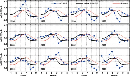
A third abiotic influence on atmospheric N2O data is the thermal signal due to

chang-ing solubility in warmchang-ing and coolchang-ing surface ocean waters. The thermal signal is max-imum in late summer in both hemispheres. It tends to oppose the observed seasonal cycle at most sites, although not at THD (Fig. 2), and thus cannot by itself explain the

15

observed cycle.

3.2 Differences among monitoring networks

N₂O data display considerable interannual variability, such that the concept of a “mean” seasonal cycle may not be very meaningful at some sites (Fig. 2). In addition, different monitoring networks that share common sites sometimes observe seasonal cycles that

20

di_ffer substantially in both shape and amplitude (Figs. 1a,b, S1, S2, Table 1). Some of the variability among networks may reflect local meteorology at the time of sampling or data filtering. To evaluate this possibility, we examined, for each month of the sea-sonal cycle, whether the detrended N₂O monthly means from different networks that share a common site showed correlated interannual variability. At Mace Head, which

25

(10)

ACPD

10, 25803–25839, 2010

signals

Title Page

Tables Figures

◭ ◮

Back Close

Full Screen / Esc

Discussion

P

a

per

|

Dis

cussion

P

a

per

|

Discussion

P

a

per

|

Discussio

n

P

a

per

by AGAGE, NOAA/CCGG and the CSIRO flask network (Fig. 1b), the detrended N₂O monthly means are significantly correlated among the three networks, although only in∼March–May around the time of the seasonal minimum, withR values around 0.7. At Barrow, Alaska, the detrended N₂O monthly means are not significantly correlated between NOAA/CCGG and in situ CATS data (Fig. S1). At the South Pole, the

de-5

trended N2O data are weakly correlated around the time of the May seasonal minimum

among the NOAA/CATS, NOAA/CCGG and CSIRO networks, although withR values only around 0.5 (Fig. S2).

The lack of correlation in detrended N2O data between NOAA/CCGG and the

AGAGE and NOAA/CATS networks at Mace Head and Barrow, respectively, could

re-10

flect limitations specific to NOAA/CCGG data. Alternatively, it could reflect the fact that interannual variability in the N2O seasonal cycle at northern sites is more strongly

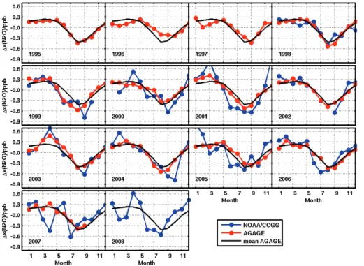
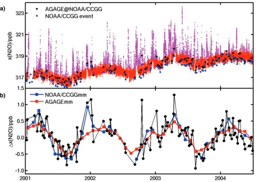
influenced by local conditions, including meteorology and pollution events, and data filtering artifacts than at southern sites. At MHD, about 20% of the in situ AGAGE mea-surements are tagged as pollution events compare to only 5% at CGO. When AGAGE

15

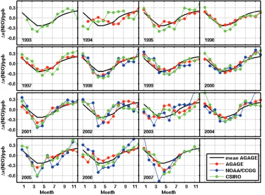
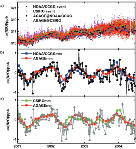
data are subsampled at MHD at the time of NOAA/CCGG flask collection, the sub-sampled dataset picks up a number of somewhat erratic features that show up in the NOAA/CCGG data, but that are smoothed out or tagged as pollution events in the full AGAGE dataset (Fig. 3a,b). At CGO, subsampling of the AGAGE data at the time of NOAA/CCGG or CSIRO flask collection can explain some of the di_fferences between

20

the full AGAGE dataset and the two flask networks (Fig. 4). However, it does not appear to be the only factor governing the discrepancies among the networks (Fig. 4b,c). In general, detecting subtle seasonal and interannual signals in N₂O data is more di_fficult for a flask network sampling every 1–2 weeks, with an average flask pair agreement of 0.4 ppb (in the case of NOAA/CCGG), than for an in situ network with a high-frequency

25

(11)

ACPD

10, 25803–25839, 2010

signals

Title Page

Tables Figures

◭ ◮

Back Close

Full Screen / Esc

Discussion

P

a

per

|

Dis

cussion

P

a

per

|

Discussion

P

a

per

|

Discussio

n

P

a

per

|

3.3 Interannual variations in the seasonal cycle

3.3.1 Northern Hemisphere

In an e_ffort to understand the causes of N₂O seasonality, we compared interannual vari-ability in the seasonal cycle to several proxies that offer mechanistic insight. The first of these proxies was mean winter polar lower stratospheric temperature. Interannual

vari-5

ation in the strength of the Brewer-Dobson circulation a_ffects the extent to which warm middle and upper stratospheric air, which is depleted in N2O and CFCs due to

pho-tolysis and oxidation, descends into the polar lower stratosphere, causing temperature to covary with N₂O and CFC minimum anomalies. The N₂O and CFC minima in turn propagate into the troposphere through stratosphere-troposphere exchange. We

inter-10

pret correlations between polar winter lower stratospheric temperature and detrended tropospheric N₂O or CFC seasonal minima as evidence of a stratospheric influence on the tropospheric seasonal cycle. However, we can not rule out the possibility that these correlations might arise if tropospheric N2O and CFC-12 variability is driven by weather

anomalies, e.g., in convection over continents, that in turn correlate with stratospheric

15

temperatures.

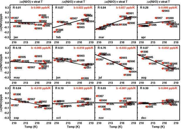
When the detrended AGAGE MHD N2O monthly means from Fig. 1a, sorted by

month, are plotted against stratospheric temperature, statistically significant anticor-relations are found in July–September, the months surrounding the August minimum (Fig. 5). Deeper minima occur during warm years, consistent with the stratospheric

20

influence hypothesized above. While the strongestR value occurs in August, a sum-mary of the monthly results shows additional significant positive correlations with strato-spheric temperature for the February-March data, near the time of the N2O maximum

and before one would expect the stratospheric influence from the current year’s Brewer-Dobson circulation to be felt in the troposphere (Fig. 6). These February-March

corre-25

(12)

ACPD

10, 25803–25839, 2010

signals

Title Page

Tables Figures

◭ ◮

Back Close

Full Screen / Esc

Discussion

P

a

per

|

Dis

cussion

P

a

per

|

Discussion

P

a

per

|

Discussio

n

P

a

per

years (Nevison et al., 2007), resulting in a flatter curve being subtracted from the raw monthly mean N₂O data in warm years.

In addition to the AGAGE N2O correlations at MHD, Fig. 7 and Table 1 show

sig-nificant correlations between mean winter polar lower stratospheric temperature and the detrended N₂O seasonal minima at ALT and BRW for CSIRO and CATS data,

re-5

spectively. At MHD, NOAA/CCGG detrended N2O minima show a weak, although not

statistically significant, anticorrelation with stratospheric temperature (Fig. 7b). Fig-ure 3b suggests that the di_fference between the AGAGE and NOAA/CCGG results at MHD may be a sampling issue, in which the relatively infrequent weekly NOAA/CCGG flask samples intersect with pollution influences and noise due to atmospheric

variabil-10

ity in the N₂O data to obscure subtle interannual signals. In support of this hypothesis, the AGAGE N2O data at MHD are themselves only weakly anticorrelated with

strato-spheric temperature when pollution-filtered monthly means are replaced with unfiltered data, with theRvalues for the detrended August monthly means dropping from 0.87 to 0.49.

15

At MHD and THD (AGAGE data), significant anticorrelations are observed between stratospheric temperature and detrended CFC-12 seasonal minima (Fig. 7e,f). At BRW, the detrended NOAA/CATS CFC-12 minima are correlated with stratospheric temperature, although the correlation is not as robust as for NOAA/CATS N2O. The

NOAA/HATS combined in situ/flask CFC-12 minima at BRW are also weakly but

signif-20

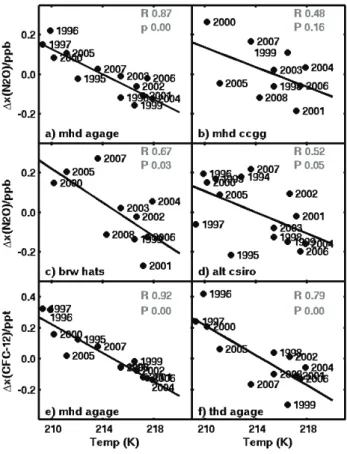
icantly correlated with stratospheric temperature for time series beginning in the 1990s and extending through the present. At MHD, where the strongest correlations with stratospheric temperature are observed for both AGAGE N₂O and CFC-12 minima, the regressions yield slopes (in ppb/K) with a ratio of about 0.7 (where CFC-12 has been normalized to N2O units by multiplying by [x(N2O)/ppb]/[x(CFC-12)/ppt]). The

25

0.7 ratio is notably similar to the Volk et al. (1996) slope of normalized N₂O vs. CFC-12 data measured near the tropopause.

(13)

ACPD

10, 25803–25839, 2010

signals

Title Page

Tables Figures

◭ ◮

Back Close

Full Screen / Esc

Discussion

P

a

per

|

Dis

cussion

P

a

per

|

Discussion

P

a

per

|

Discussio

n

P

a

per

|

September), although additional correlations in the months surrounding the minimum also occur in some cases. The correlation coefficients in Fig. 7 and Table 1 indicate that the interannual variability in the stratospheric signal can account for anywhere between

∼75% (at MHD) and∼25% (at ALT) of the variability in the detrended minima. Noise in

the data, biogeochemical sources and tropospheric transport variability, especially at

5

high latitudes, may account for the remainder.

Trinidad Head, California is an interesting case in which the detrended CFC-12 monthly means are significantly anticorrelated to stratospheric temperature in August, but the detrended N2O monthly means are not (Fig. 8a,c). Since N2O data at THD

are known to be influenced by ventilation of N₂O-enriched deepwater during coastal

10

upwelling events (Lueker et al., 2003), we performed additional regressions of THD detrended N2O data against the coastal upwelling index for the Pacific Northwest.

Cor-relations of R=0.45 to 0.66 were found in April–September (the upwelling season), with more positive N₂O values occurring during years of strong upwelling (Fig. 8b). A multivariate regression of detrended N2O data against the upwelling index and

15

stratospheric temperature improved these correlations to R=0.64 to 0.82 for April– September (Fig. 8d). Statistically significant correlations were obtained from the multi-variate regression using the coastal upwelling indices at 42◦N, 45◦N and 48◦N (THD is at 40◦N), with best results obtained for the 45◦N index. The results at THD indicate that sites located near strong regional N₂O sources are also substantially a_ffected by

20

the stratospheric influx and that the latter influence must be accounted for in order to best interpret the biogeochemical signal in monthly mean data.

3.3.2 Southern Hemisphere

In previous studies, the stratospheric influence on N₂O and CFC-12 has been less clear in the Southern Hemisphere than in the Northern Hemisphere. Two atmospheric

gen-25

(14)

ACPD

10, 25803–25839, 2010

signals

Title Page

Tables Figures

◭ ◮

Back Close

Full Screen / Esc

Discussion

P

a

per

|

Dis

cussion

P

a

per

|

Discussion

P

a

per

|

Discussio

n

P

a

per

although both models predicted a coherent signal in summer in the Northern Hemi-sphere (Nevison et al., 2004; Ishijima et al., 2010). In contrast, the GEOS CCM model predicted coherent cycles in CFC-12 with autumn minima (Liang et al., 2008), although the amplitudes were about 50% smaller than the corresponding Northern Hemisphere amplitudes. Isotopic evidence, i.e., seasonal enrichment in15N-N₂O characteristic of

5

stratospheric air, also provides support for a stratospheric signal in tropospheric N2O

at CGO (Park et al., 2008). In addition, N2O and CFC-12 seasonal cycles and

inter-annual growth rate anomalies at Cape Grim are generally well correlated, suggesting a common influence such as the stratospheric influx (Nevison et al., 2004, 2007).

Stratosphere-troposphere exchange (STE) in the Southern Hemisphere is not as

10

well studied as in the Northern Hemisphere, although it is thought to be coupled to a Brewer-Dobson circulation with weaker, less strongly seasonal descent into the win-ter pole than in the Northern Hemisphere (Holton et al., 1995). The polar vortex is also more stable and persistent in the Southern Hemisphere, which traps N₂O and CFC-depleted air in the polar lower stratosphere longer and hinders exchange with

15

mid-latitudes, where most STE occurs, until late spring or early summer (Nevison et al., 2007). The late polar vortex breakup, combined with a lower-stratosphere-to-surface propagation time of several months for the stratospheric signal, may explain the later minima (autumn vs. late summer) observed in the Southern vs. Northern Hemispheres (Nevison et al., 2004; Liang et al., 2008).

20

The detrended AGAGE N₂O monthly means at Cape Grim (Fig. 1b), sorted by month and plotted against austral polar lower stratospheric temperature from the previous winter-spring, show statistically significant anticorrelations in January–February, with more negative values occurring during warm years. By May–June, however, the de-trended N2O data become positively correlated to stratospheric temperature (Fig. 9).

25

(15)

ACPD

10, 25803–25839, 2010

signals

Title Page

Tables Figures

◭ ◮

Back Close

Full Screen / Esc

Discussion

P

a

per

|

Dis

cussion

P

a

per

|

Discussion

P

a

per

|

Discussio

n

P

a

per

|

stratospheric temperature are found for AGAGE CFC-12 (Fig. 10a).

In an effort to better understand these findings, and because the N2O minimum at

CGO varies from February-June in individual years, most commonly occuring in April or May (Fig. 1b), we regressed the month of the AGAGE N₂O minimum against polar vortex break-up date (ranging from mid-November to the end of December) and found

5

that earlier minima tended to occur in years with early vortex breakup and later minima in years with late breakup (R=0.75). However, warmer stratospheric temperatures are themselves significantly correlated with earlier vortex breakup (R=0.79), such that the two indices provide more or less redundant, rather than independent, predictive capability for the detrended N₂O monthly means.

10

The NOAA/CCGG flask data at CGO show correlation patterns with stratospheric temperature that are similar to those seen by AGAGE, although the correlations are statistically significant only in January (Fig. 10d, e). In addition, both the NOAA/CCGG and CSIRO flask networks show correlation patterns similar to those seen at CGO by AGAGE at many of their other extratropical southern sites (Fig. 11, Table 1). In

15

most cases, the anticorrelations are strongest in the months preceding the N2O

mini-mum, which typically occurs in May, with the exception of Macquarie Island, where the anticorrelation is strongest in May. At the South Pole, neither the CSIRO, CATS nor NOAA/CCGG networks shows statistically significant correlations between detrended N₂O data and stratospheric temperature, although there is a hint of an anticorrelation

20

in January–February in detrended CATS CFC-12 data (Table 1). Since STE of N2

O-depleted air takes place mainly at midlatitudes (Ishijima et al., 2010), the South Pole site is more poorly situated then the other sites to detect the stratospheric signal.

The mixed results in Figs. 9–11 suggest that the stratospheric influx following polar vortex breakup does exert a coherent influence on the N2O seasonal cycle, but that this

25

(16)

ACPD

10, 25803–25839, 2010

signals

Title Page

Tables Figures

◭ ◮

Back Close

Full Screen / Esc

Discussion

P

a

per

|

Dis

cussion

P

a

per

|

Discussion

P

a

per

|

Discussio

n

P

a

per

(Figs. 2, 8).

Like Trinidad Head, monitoring sites in the Southern Ocean region are influenced by ventilation of oceanic, microbially-produced N2O. This is especially true of sites

situated in the heart of the Antarctic Circumpolar Current (Orsi et al., 1995), between

∼50◦–60◦S, where strong winds and upwelling lead to deep ventilation of N₂O-enriched

5

subsurface waters . Nevison et al. (2005) hypothesized that the N2O seasonal cycle at

Cape Grim can be decomposed into comparable contributions from ocean ventilation, the stratospheric influx, and an abiotic thermal signal due to warming and cooling of surface waters (Fig. 12a). The stratospheric signal in Fig. 12a is estimated based on the observed, normalized CFC-12 cycle at CGO multiplied by a scaling factor which is

10

uncertain, but which we assign a best guess value of 0.7 based on the discussion in Sect. 3.3.1.

Unlike THD, where the thermal signal is in phase with the summer upwelling N2O

source, ventilation of Southern Ocean waters occurs during the breakdown of the sea-sonal thermocline in fall and winter, and thus opposes the thermal signal. In Fig. 12b,

15

the thermally-corrected N2O cycle, i.e., subtracting the estimated thermal signal from

the observed “mean” seasonal cycle, yields a cycle that closely resembles the ob-served CFC-12 cycle. (CFC-12 also experiences thermal ingassing and outgassing, but is 8 times less soluble than N2O, such that the thermal correction has little impact

on its cycle (Fig. 12b).) The ocean ventilation and stratospheric signals are roughly

20

coincident, with the former a positive signal peaking in early fall and the latter a neg-ative signal peaking in spring, making the two signals difficult to distinguish based on mixing ratio data alone. Indeed, the possibility that the thermally-corrected N₂O cycle in Fig. 12b is primarily or entirely due to the stratospheric influx with no influence from ocean ventilation cannot be ruled out, although this is inconsistent with evidence from

25

atmospheric O₂/N₂ data and ocean biogeochemistry models (Jin and Gruber, 2003; Nevison et al., 2005).

(17)

ACPD

10, 25803–25839, 2010

signals

Title Page

Tables Figures

◭ ◮

Back Close

Full Screen / Esc

Discussion

P

a

per

|

Dis

cussion

P

a

per

|

Discussion

P

a

per

|

Discussio

n

P

a

per

|

may be stronger at sites further poleward, in the upwelling region. We tested this hypothesis (following the example at THD) by regressing detrended N₂O monthly mean flask data at several Southern Hemisphere sites against a multivariate combination of stratospheric temperature and zonally-averaged NCEP wind speed or windstress curl at the latitude band of the site (Kalnay et al., 1996). Although no significant correlations

5

were found, a more judicious or focused proxy for ocean ventilation, combined with an in situ N2O record at a site within the upwelling region, arguably might yield better

results. In addition, it may be necessary to account for interannual variability in the thermal signal, which directly competes with the ventilation signal.

4 Conclusions

10

Correlations between detrended tropospheric N₂O monthly mean data, sorted by month, and various interannually-varying proxies, including polar lower stratospheric temperature, polar vortex breakup date and coastal upwelling indices, are used to help identify the mechanisms that cause interannual variability in the N₂O seasonal cycle. In the months surrounding the N2O seasonal minimum, the detrended N2O data are

15

significantly anti-correlated with winter polar lower stratospheric temperature at a num-ber of Northern Hemisphere surface monitoring sites, with deeper minima occurring in warm years, providing strong empirical evidence that these seasonal cycles bear a stratospheric influence. At Trinidad Head, California, detrended N2O monthly means

in summer are weakly correlated to the index for coastal upwelling, which ventilates

20

N2O-enriched deepwater to the atmosphere, but more strongly correlated after the

stratospheric influence is accounted for using a multivariate regression against both stratospheric temperature and the coastal upwelling index. Monitoring sites in the ex-tratropical Southern Hemisphere, where the stratospheric influence on surface N2O

has been more difficult to establish in previous studies, also show anti-correlations

25

(18)

ACPD

10, 25803–25839, 2010

signals

Title Page

Tables Figures

◭ ◮

Back Close

Full Screen / Esc

Discussion

P

a

per

|

Dis

cussion

P

a

per

|

Discussion

P

a

per

|

Discussio

n

P

a

per

seasonal minimum as in the northern hemisphere, but rather are stronger in months preceding the minimum. Southern Ocean sites also are likely influenced by oceanic thermal and biological ventilation signals, but these influences are difficult to prove using the methodology of this study. N2O seasonal cycles can vary strongly year to

year, making a “mean” cycle difficult to define at some sites, especially those subject

5

to competing influences from various interannually-varying sources and sinks. Among networks that share a common site, interannual variability in detrended N2O monthly

means is not necessarily well correlated, especially in the Northern Hemisphere. In part, this is a sampling issue, with weekly flask networks less able to detect subtle in-terannual signals and filter out noise due to atmospheric variability than more frequently

10

sampled in situ networks. Due to the various abiotic influences on N₂O seasonal cycles, including thermal oceanic in and outgassing, stratospheric influx, and tropo-spheric transport, sites that measure a complementary tracer, e.g.,15N-N2O or

CFC-12, that helps separate transport and stratospheric influences from soil and oceanic biogeochemical source signals are more likely to provide insight into seasonality in

15

N2O sources.

Supplementary material related to this article is available online at: http://www.atmos-chem-phys-discuss.net/10/25803/2010/

acpd-10-25803-2010-supplement.pdf.

Acknowledgement. CDN acknowledges support from NASA grant NNX08AB48G and thanks

20

Paul Newman and Eric Nash for stratospheric data and Qing Liang and Ralph Keeling for help-ful comments. The authors are deeply gratehelp-ful to the many people, from many organisations around the world, who have contributed to the production of the excellent N₂O datasets that have made this study possible. These include the people who diligently collect flask air sam-ples, those who analyze the flask samsam-ples, and those sta_ffwho maintain the optimal operation

25

(19)

ACPD

10, 25803–25839, 2010

signals

Title Page

Tables Figures

◭ ◮

Back Close

Full Screen / Esc

Discussion

P

a

per

|

Dis

cussion

P

a

per

|

Discussion

P

a

per

|

Discussio

n

P

a

per

|

References

Forster, P., Ramaswamy, V., Artaxo, P., Berntsen, T., Betts, R., Fahey, D. W., Haywood, J., Lean, J., Lowe, D. C., Myhre, G., Nganga, J., Prinn, R., Raga, G., Schulz, M., and Van Dorland, R.: Changes in atmospheric constituents and in radiative forcing, in: Climate Change 2007: The Physical Science Basis. Contribution of Working Group I to the Fourth

As-5

sessment Report of the Intergovernmental Panel on Climate Change. Cambridge University Press Cambridge, UK and New York, NY, USA, 2007.

Francey, R. J., Steele, L. P., Spencer, D. A., Langenfelds, R. L., Law, R. M., Krummel, P. B., Fraser, P. J., Etheridge, D. M., Derek, N., Coram, S. A., Cooper, L. N., Allison, C. E., Porter, L., and Baly, S.: The CSIRO (Australia) measurement of greenhouse gases in the global

atmo-10

sphere, in: Baseline Atmospheric Program Australia 1999–2000, edited by: Tindale, N. W., Derek, N., and Fraser, P. J., Bureau of Meteorology and CSIRO Atmospheric Research, Melbourne, Australia, 42–53, 2003.

Glatthor, N., et al.: Mixing processes duing the Antarctic vortex split in September–October 2002 as inferred from source gas and ozone distributions from ENVISAT-MIPAS, J. Atmos.

15

Sci., 62(3), 787–800, 2005.

Gettelman, A. and Sobel, A. H.: Direct diagnoses of stratosphere-troposphere exchange, J. At-mos. Sci., 57(1), 3–16, 2000.

Hirsch, A. I., Michalak, A. M., Bruhwiler, L. M., Peters, W., Dlugokencky, E. J., and Tans, P. P.: Inverse modeling estimates of the global nitrous oxide surface flux from 1998–2001, Global

20

Biogeochem. Cy., 20, GB1008, 2006.

Holton, J. R., Haynes, P. H., McIntyre, M. E., Douglass, A. R., Rood, R. B., and Pfister, L.: Stratosphere-troposphere exchange, Rev. Geophys., 33(4), 403–439, 1995.

Huang, J., Golombek, A., Prinn, R., Weiss, R., Fraser, P., Simmonds, P., Dlugokencky, E. J., Hall, B., Elkins, J., Steele, P., Langenfelds, R., Krummel, P., Dutton, G., and Porter, L.:

Esti-25

mation of regional emissions of nitrous oxide from 1997 to 2005 using multinetwork measure-ments, a chemical transport model, and an inverse method, J. Geophys. Res. 113, D17313, doi:10.1029/2007JD009381, 2008.

Ishijima, K., Nakazawa, T., Sugawara, S., Aoki, S., and Saeki, T.: Concentration variations of tropospheric nitrous oxide over Japan, Geophys. Res. Lett., 28(1), 171–174, 2001.

30

(20)

ACPD

10, 25803–25839, 2010

signals

Title Page

Tables Figures

◭ ◮

Back Close

Full Screen / Esc

Discussion

P

a

per

|

Dis

cussion

P

a

per

|

Discussion

P

a

per

|

Discussio

n

P

a

per

the seasonal cycle of nitrous oxide in the troposphere as deduced from aircraft observations and model simulations, J. Geophys. Res., doi:10.1029/2009JD013322, 2010.

Jiang, X., Ku, W. L., Shia, R.-L., Li, Q., Elkins, J. W., Prinn, R. G., and Yung, Y. L.: Seasonal cycle of N₂O: analysis of data, Global Biogeochem. Cy., 21, GB1006, 2007.

Jin, X. and Gruber, N.: Offsetting the radiative benefit of ocean iron fertilization by enhancing

5

N₂O emissions, Geophys. Res. Lett., 30(24), 2249, 2003.

Jin, X., Najjar, R. G., Louanchi, F., and Doney, S. C.: A modeling study of the seasonal oxygen budget of the global ocean, J. Geophys. Res., 112, C05017, doi:10.1029/2006JC003731, 2007.

Kalnay, E., Kanamitsu, M., Kistler, R., Collins, W., Deaven, D., et al.: The NMC/NCAR 40-year

10

reanalysis project, B. Am. Meteorol. Soc., 77, 437–471, 1996.

Kroeze, C., Mosier, A., and Bouwman, L.: Closing the global N₂O budget: A retrospective analysis 1500–1994, Global Biogeochem. Cy., 13, 1–8, 1999.

Liang, Q., Stolarski, R. S., Douglass, A. R., Newman, P. A., and Nielsen, J. E.: Evaluation of emissions and transport of CFCs using surface observations and their seasonal

cy-15

cles and the GEOS CCM simulation with emissions-based forcing, J. Geophys. Res., 113, doi:10.1029/2007JD009617, 2008.

Liang, Q., Douglass, A. R., Duncan, B. N., Stolarski, R. S., and Witte, J. C.: The governing processes and timescales of stratosphere-to-troposphere transport and its contribution to ozone in the Arctic troposphere, Atmos. Chem. Phys., 9, 3011–3025,

doi:10.5194/acp-9-20

3011-2009, 2009.

Liao, T., Camp, C. D., and Yung, Y. L.: The seasonal cycle of N₂O, Geophys. Res. Lett., 31, 17108, 2004.

Levin, I. P., Cias, P., Langenfelds, R., Schmidt, M., Ramonet, M., et al.: Three years of trace gas observations over the EuroSiberian domain derived from aircraft sampling – a concerted

25

action, Tellus, 54B, 696–712, 2002.

Lueker, T. J., Walker, S. J., Vollmer, M. K., Keeling, R. F., Nevison, C. D., and Weiss, R. F.: Coastal upwelling air-sea fluxes revealed in atmospheric observations of O₂/N₂, CO₂ and N₂O, Geophys. Res. Lett., 30, 1292, 2003.

MacFarling Meure, C., Etheridge, D. M., Trudinger, C. M., Steele, L. P., Langenfelds, R. L., van

30

Ommen, T., Smith, A., and Elkins, J. W.: Law Dome CO₂, CH₄, and N₂O ice core records extended to 2000 years BP, Geophys. Res. Lett., 33, L14810, 2006.

(21)

ACPD

10, 25803–25839, 2010

signals

Title Page

Tables Figures

◭ ◮

Back Close

Full Screen / Esc

Discussion

P

a

per

|

Dis

cussion

P

a

per

|

Discussion

P

a

per

|

Discussio

n

P

a

per

|

radon-222 to the remote troposphere using the Model of Atmospheric Transport and Chem-istry and assimilated winds from ECMWF and the National Center for Environmental Predic-tion/NCAR, J. Geophys. Res., 102, 28139–28151, 1997.

Mosier, A. R., Duxbury, J. M., Freney, J. R., Heinemeyer, O., and Minami, K.: Assessing and mitigating N₂O emissions from agricultural soils, Climatic Change, 40, 7–38, 2000.

5

Nevison, C. D., Kinnison, D. E., and Weiss, R. F.: Stratospheric Influence on the tropospheric seasonal cycles of nitrous oxide and chlorofluorocarbons, Geophys. Res. Lett., 31(20), L20104, 2004.

Nevison, C. D., Keeling, R. F., Weiss, R. F., Popp, B. N., Jin, X., Fraser, P. J., Porter, L. W., and Hess, P. G.: Southern Ocean ventilation inferred from seasonal cycles of atmospheric N₂O

10

and O₂/N₂at Cape Grim, Tasmania, Tellus, 57B, 218–229, 2005.

Nevison, C. D., Mahowald, N. M., Weiss, R. F., and Prinn, R. G.: Interannual and seasonal variability in atmospheric N₂O, Global Biogeochem. Cy., 21, GB3017, 2007.

Orsi, A. H., Whitworth III, T., and Nowlin Jr., W. D.: On the meridional extent and fronts of the Antarctic Circumpolar Current, Deep-Sea Res. Pt. I, 42(5), 651–673, 1995.

15

Park, S., Boering, K. A., and Etheridge, D. M.: Trends, seasonal cycles, and interannual variabil-ity in the isotopic composition of nitrous oxide between 1940 and 2008, Eos Trans., 89(53), Abstract A21A-0125, 2008.

Prinn, R. G., Weiss, R. F., Fraser, P. J., Simmonds, P. G., Cunnold, D. M., Alyea, F. N., O’Doherty, S., Salameh, P., Miller, B. R., Huang, J., Wang, R. H. J., Hartley, D. E., Harth, C.,

20

Steele, L. P., Sturrock, G., Midgley, P. M., and McCulloch, A.: A history of chemically and radiatively important gases in air deduced from ALE/GAGE/AGAGE, J. Geophy. Res., 105(D14), 17751–17792, 2000.

Ravishankara, A. R., Daniel, J. S., and Portmann, R. W.: Nitrous oxide (N₂O): The dom-inant ozone depleting substance emitted in the 21st century, Science, 326, 123–125,

25

doi:10.1126/science.1176985, 2009.

Sokal, R. R. and Rohlf, F. J.: Biometry, W. H. Freeman, New York, USA, 859 pp., 1981.

Thompson, T. M., Elkins, J. W., Hall, B., et al.: Halocarbons and other atmospheric trace species, in: Climate Diagnostics Laboratory Summary Report #27, 2002–2003, edited by: Schnell, R. C., Buggle, A.-M., and Rossson, R. M., US Department of Commerce, National

30

Oceanic and Atmospheric Administration, Boulder, Colorado, 2004.

(22)

ACPD

10, 25803–25839, 2010

signals

Title Page

Tables Figures

◭ ◮

Back Close

Full Screen / Esc

Discussion

P

a

per

|

Dis

cussion

P

a

per

|

Discussion

P

a

per

|

Discussio

n

P

a

per

Chan, K. R.: Quantifying transport between the tropical and mid-latitude lower stratosphere, Science, 272, 1763–1768, 1996.

(23)

ACPD

10, 25803–25839, 2010

signals

Title Page

Tables Figures

◭ ◮

Back Close

Full Screen / Esc

Discussion

P

a

per

|

Dis

cussion

P

a

per

|

Discussion

P

a

per

|

Discussio

n

P

a

per

|

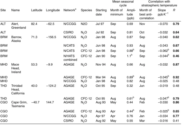
Table 1. Correlations between N₂O seasonal minimum anomalies and mean polar (60◦–90◦) lower stratospheric (at 100 hPa) temperature for January–March (Northern Hemisphere) or September–November (Southern Hemisphere). Bold type in final column indicates statistically significant correlations (p≤0.05).

Mean seasonal Correlation with cycle stratospheric temperature Site Name Latitude Longitude Networka Species Starting Month of Ampli- Month of Slope R

date minimum tude best anti- ppb K−1

(ppb) correlation

ALT Alert, 82.4 −62.5 N/CCGG N2O Jul 97 Sep 0.69 Nov −0.070 0.79

Greenland

ALT CSIRO N2O Jul 92 Sep 0.81 Oct −0.032 0.64

BRW Barrow, 71.3 −156.5 N/CCGG N2O Jan 98 Aug 0.87 Sep −0.040 0.62

Alaska

BRW N/CATS N2O Jun 98 Aug 0.93 Aug −0.043 0.67

BRW N/CATS CFC-12 Jun 98 Sep 0.88b Sep −0.062b 0.66

BRW N/HATS CFC-12 Jan 90 Sep 1.1b Sep −0.044b 0.46

combined

MHD Mace 53.3 −9.9 AGAGE N2O Nov 94 Aug 0.66 Aug −0.032 0.87

Head, Ireland

MHD AGAGE CFC-12 Mar 94 Aug 0.89b Aug −0.045b 0.92

MHD N/CCGG N2O Jan 98 Aug 0.82 Aug −0.025 0.48

THD Trinidad 40.0 −124.2 AGAGE N2O Oct 95 Sep 0.32 Jun −0.019 0.48

Head, California

THD AGAGE CFC-12 Oct 95 Aug 0.61b Aug −0.047b 0.79

CGO Cape Grim, −40.7 144.7 AGAGE N2O Aug 93 May 0.44 Feb −0.030 0.86

Tasmania

CGO AGAGE CFC-12 Aug 93 Apr 0.44b Feb −0.025b 0.65

CGO N/CCGG N2O Apr 97 Apr 0.76 Jan −0.034 0.77

(24)

ACPD

10, 25803–25839, 2010

signals

Title Page

Tables Figures

◭ ◮

Back Close

Full Screen / Esc

Discussion

P

a

per

|

Dis

cussion

P

a

per

|

Discussion

P

a

per

|

Discussio

n

P

a

per

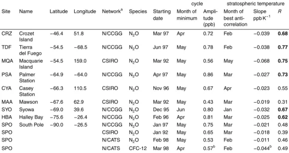
Table 1.Continued.

Mean seasonal Correlation with cycle stratospheric temperature Site Name Latitude Longitude Networka Species Starting Month of Ampli- Month of Slope R

date minimum tude best anti- ppb K−1

(ppb) correlation

CRZ Crozet −46.4 51.8 N/CCGG N2O Mar 97 Apr 0.72 Feb −0.039 0.68

Island

TDF Tierra −54.5 −68.5 N/CCGG N2O Jun 97 May 0.78 Feb −0.038 0.77

del Fuego

MQA Macquarie −54.5 159.0 CSIRO N2O Mar 92 May 0.56 May −0.068 0.75

Island

PSA Palmer −64.9 −64.0 N/CCGG N2O Apr 97 May 0.86 Mar −0.027 0.73

Station

CYA Casey −66.3 110.5 CSIRO N2O Nov 96 May 0.67 Apr −0.023 0.55

Station

MAA Mawson −67.6 62.9 CSIRO N2O Mar 92 May 0.43 Mar −0.019 0.31

SYO Syowa −69.0 39.6 N/CCGG N2O Dec 95 Jun 0.80 Jan −0.032 0.67

HBA Halley Bay −75.6 −26.4 N/CCGG N2O Feb 96 Apr 0.81 Mar −0.025 0.62

SPO South Pole −90.0 −26.5 N/CCGG N2O Jan 97 May 0.75 Mar −0.021 0.48

SPO CSIRO N2O Jan 92 May 0.65 Mar −0.018 0.39

SPO N/CATS N2O Feb 98 May 0.53 Feb −0.011 0.46

SPO N/CATS CFC-12 Mar 98 Apr 0.57b _Feb ₋_0.044b _0.49

a_{NOAA/CCGG, NOAA/HATS and NOAA/CATS abbreviated as N/CCGG, N/HATS and N/CATS;} b_{CFC-12 slopes and mean seasonal amplitudes are normalized to N}

(25)

ACPD

10, 25803–25839, 2010

signals

Title Page

Tables Figures

◭ ◮

Back Close

Full Screen / Esc

Discussion

P

a

per

|

Dis

cussion

P

a

per

|

Discussion

P

a

per

|

Discussio

n

P

a

per

|

(26)

ACPD

10, 25803–25839, 2010

signals

Title Page

Tables Figures

◭ ◮

Back Close

Full Screen / Esc

Discussion

P

a

per

|

Dis

cussion

P

a

per

|

Discussion

P

a

per

|

Discussio

n

P

a

per

(27)

ACPD

10, 25803–25839, 2010

signals

Title Page

Tables Figures

◭ ◮

Back Close

Full Screen / Esc

Discussion

P

a

per

|

Dis

cussion

P

a

per

|

Discussion

P

a

per

|

Discussio

n

P

a

per

|

(28)

ACPD

10, 25803–25839, 2010

signals

Title Page

Tables Figures

◭ ◮

Back Close

Full Screen / Esc

Discussion

P

a

per

|

Dis

cussion

P

a

per

|

Discussion

P

a

per

|

Discussio

n

P

a

per

a)

b)

(29)

ACPD

10, 25803–25839, 2010

signals

Title Page

Tables Figures

◭ ◮

Back Close

Full Screen / Esc

Discussion

P

a

per

|

Dis

cussion

P

a

per

|

Discussion

P

a

per

|

Discussio

n

P

a

per

|

a)

b)

c)

(30)

ACPD

10, 25803–25839, 2010

signals

Title Page

Tables Figures

◭ ◮

Back Close

Full Screen / Esc

Discussion

P

a

per

|

Dis

cussion

P

a

per

|

Discussion

P

a

per

|

Discussio

n

P

a

per

(31)

ACPD

10, 25803–25839, 2010

signals

Title Page

Tables Figures

◭ ◮

Back Close

Full Screen / Esc

Discussion

P

a

per

|

Dis

cussion

P

a

per

|

Discussion

P

a

per

|

Discussio

n

P

a

per

|

a)

b)

(32)

ACPD

10, 25803–25839, 2010

signals

Title Page

Tables Figures

◭ ◮

Back Close

Full Screen / Esc

Discussion

P

a

per

|

Dis

cussion

P

a

per

|

Discussion

P

a

per

|

Discussio

n

P

a

per

Fig. 7.Detrended N₂O residuals at the minimum month in the mean annual cycle (September for Alert, August for the other sites) vs. polar winter lower stratospheric temperature, N₂O(a–d)

(33)

ACPD

10, 25803–25839, 2010

signals

Title Page

Tables Figures

◭ ◮

Back Close

Full Screen / Esc

Discussion

P

a

per

|

Dis

cussion

P

a

per

|

Discussion

P

a

per

|

Discussio

n

P

a

per

|

(34)

ACPD

10, 25803–25839, 2010

signals

Title Page

Tables Figures

◭ ◮

Back Close

Full Screen / Esc

Discussion

P

a

per

|

Dis

cussion

P

a

per

|

Discussion

P

a

per

|

Discussio

n

P

a

per

(35)

ACPD

10, 25803–25839, 2010

signals

Title Page

Tables Figures

◭ ◮

Back Close

Full Screen / Esc

Discussion

P

a

per

|

Dis

cussion

P

a

per

|

Discussion

P

a

per

|

Discussio

n

P

a

per

|

(36)

ACPD

10, 25803–25839, 2010

signals

Title Page

Tables Figures

◭ ◮

Back Close

Full Screen / Esc

Discussion

P

a

per

|

Dis

cussion

P

a

per

|

Discussion

P

a

per

|

Discussio

n

P

a

per

Fig. 11. Stem plots summarizing the linear regression slopes for detrended N₂O monthly means at 8 different Southern Hemisphere sites spanning 3 monitoring networks vs. mean southern polar winter–spring lower stratospheric temperature. Heavy lines indicate statistically significant correlations at the 5% confidence level, with darker lines, signifying higherR val-ues. Medium grey lines with open circles indicate marginally significant correlations at 10% confidence level: (a) Crozet Island (NOAA/CCGG), (b)Tierra del Fuego (NOAA/CCGG), (c)

Macquarie Island (CSIRO),(d)Palmer Station (NOAA/CCGG),(e)Casey Station (CSIRO),(f)

(37)

ACPD

10, 25803–25839, 2010

signals

Title Page

Tables Figures

◭ ◮

Back Close

Full Screen / Esc

Discussion

P

a

per

|

Dis

cussion

P

a

per

|

Discussion

P

a

per

|

Discussio

n

P

a

per

|

a) b)

Fig. 12. (a)Decomposition of N₂O seasonal cycle at Cape Grim based on methodology de-scribed in Nevison et al. (2005). Envelopes show estimated uncertainty in stratospheric and thermal signals, with the biological oceanic ventilation signal derived as a residual of observed N₂O minus the thermal and stratospheric terms. Figure uses smoothed, idealized curves.