Causal Theory of Relativistic Dissipative Hydrodynamics
G. S. Denicol, T. Kodama, T. Koide, and Ph. Mota
Instituto de F´ısica, Universidade Federal do Rio de Janeiro, C. P. 68528, 21945-970, Rio de Janeiro, Brazil
Received on 10 November, 2006
We present a new formalism for the theory of relativistic dissipative hydrodynamics, where covariance and causality are satisfied by introducing the memory effect in irreversible currents. Our theory has a much simpler structure and thus has several advantages for practical purposes compared to the Israel-Stewart theory (IS). We apply our formalism to the Bjorken model and the results are shown to be analogous to the IS.
Keywords: Causality; Dissipation; Hydrodynamics
I. INTRODUCTION
The ideal hydrodynamical description for the dynamics of hot and dense matter achieved in RHIC experiments works amazingly well, particularly for the behavior of collective flow parameters. Together with other signals, the success of the approach is considered as the indication of the emergence of a new state of strongly interacting matter, the plasma of quarks and gluons (QGP). The comparison between RHIC and SPS results shows that this new state of matter is formed at the very early stage of the relativistic heavy ion collisions for RHIC energies.
However, we know that there still exist several open prob-lems in the interpretation of data in terms of the hydrodynami-cal model [1]. These questions require careful examination to extract quantitative and precise information on the properties of QGP. In particular, we should study the effect of dissipative processes on collective flow variables. Several works have been done in this direction [2]. However, strictly speaking, a quantitative and consistent analysis of the viscosity within the framework of relativistic hydrodynamics has not yet been done completely. This is because the introduction of dissi-pative phenomena in relativistic hydrodynamics casts difficult problems, both conceptual and technical. Initially Eckart, and later, Landau-Lifshitz introduced the dissipative effects in rel-ativistic hydrodynamics in a covariant manner [3, 4]. It is, however, known that their formalism leads to the problem of non-causality, that is, a pulse signal propagates with infinite speed. Thus, relativistic covariance is not a sufficient condi-tion for a consistent relativistic dissipative dynamics [5, 6].
To cure this problem, relativistic hydrodynamics in the framework of extended thermodynamics was developed by M¨uller [7] and later by Israel and Stewart [8–10]. From the kinetic point of view [11], this formalism corresponds to the extension of equilibrium thermodynamics to include the sec-ond order moments of kinetic variables. This is the reason why this theory is usually refereed to as the second order the-ory. However, it is known that the Israel-Stewart theory (IS) is not the unique approach to relativistic dissipative hydro-dynamics. To the authors’ knowledge, there is at least one other causal theory called the divergence type [12–16]. In this work, we present a very simple alternative theory which sat-isfies the minimal conditions mentioned above. We show that the causality problem of the Landau-Lifshitz formalism (LL) can be solved by introducing a memory effect. This memory
effect is characterized by the relaxation timeτR, so that our theory introduces only one additional parameter to the usual bulk viscosity, shear viscosity and thermal conduction coeffi-cients of the Navier-Stokes equation. Our theory recovers the relativistic Navier-Stokes equation in the limit of vanishing values of this relaxation time.
As described later more in detail, our approach has a funda-mental advantage from the practical point of view in addition to its physical simplicity. The dissipative terms are explic-itly given by the integral of the independent variables of the usual ideal hydrodynamics. Thus, the implementation of our method to the existing ideal hydro-codes is straightforward, particularly, to those based on the local Lagrangian coordinate system such as SPheRIO [17, 18].
The present paper is organized as follows. In the next sec-tion, we briefly review the problem of non-causal propagation in the diffusion equation and the method to cure this problem in terms of the memory effect, which leads to the so-called telegraphist’s equation. In the Sec. III, we analyze the struc-ture of the LL of relativistic dissipative hydrodynamics and introduce the memory effect to solve the non-causal problem due to its parabolic nature. We thus obtain the dissipative hy-drodynamical equations with the minimum number of para-meters which satisfies causality. In Sec. IV, we discuss the problem of entropy production in our formalism. In Sec. V, we discuss the propagation speed of our equation. In Sec.VI, we apply our equation to the Bjorken solution, and compare with the previous analysis [19–23]. In Sec. VII, we summa-rize our results and discuss possible immediate applications.
II. DIFFUSION EQUATION AND ACAUSALITY
The fundamental problem of first-order theories, like the Navier-Stokes theory, is attributed to the fact that the diffu-sion equation is parabolic. The diffudiffu-sion process is a typical relaxation process of conserved quantities. Thus, it should satisfy the equation of continuity,
∂n
∂t +∇·j=0, (1)
n,
j=−ζF=−ζ∇n, (2) where the Onsager coefficient ζ. Substituting Eq.(2) into Eq.(1), we get the diffusion equation,
∂ ∂tn=ζ∇
2n. (3)
Fick’s law tells us that the above diffusion process is in-duced by an inhomogeneous distribution. In Eq.(2), the space inhomogeneity immediately gives rise to the irreversible cur-rent. However, this is a very idealized case. In general, the generation of irreversible currents has a time delay. Thus, we may think of memory effects by introducing the follow-ing memory function [26–28],
Gt,t′ = 1
τRe
−(t−t′)/τR, t≥t′
=0, t<t′ (4)
whereτRcharacterizes the memory time and called the relax-ation time. Then, we rewrite Eq.(2) as
j=−
t
−∞
Gt,t′ζFt′dt′. (5) In the limit ofτR→0,we haveG(t,t′)→δ(t−t′)so that the original equation (2) is recovered [29]. Substituting into the equation of continuity (1), we arrive at
τR ∂2n ∂t2 = −
∂n
∂t +ζ∇ 2n.
(6)
This equation is hyperbolic. This telegraph equation is some-times called the causal diffusion equation.
The maximum velocity of the signal propagation of the causal diffusion equation is [25],
vmax=
ζ τR
. (7)
For a suitable choice of the parametersτR andζ, we can recover causal propagation of the diffusion process. On the other hand, the diffusion equation corresponds toτR=0 and hencevmax→∞. This is the reason why the diffusion equation breaks causality.
III. RELATIVISTIC DISSIPATIVE HYDRODYNAMICS
Eckart and Landau-Lifshitz derived relativistic dissipative hydrodynamics following non-equilibrium thermodynamics as discussed in the preceding section [3, 4]. Their theories are just the covariant versions of the Navier-Stokes equation and the corresponding equations still continue to be parabolic. Therefore, they do not satisfy causality and some modification should be required. In the IS and the divergence type theory, the definition of the entropy four-flux is generalized and, to
satisfy the second law of thermodynamics, modified thermo-dynamic forces are obtained. In this section, we propose an-other approach, where the problem of non-causality is solved by introducing the memory effect as was done in Eq. (5) [30]. For this purpose, let us first analyze briefly the structure of the LL. The hydrodynamical equation of motion is written as the conservation of the energy-momentum tensor ,
∂µTµν=0, (8)
together with the conservation of a quantity, for example, the baryon number,
∂µNµ=0. (9)
In the LL, it is assumed that thermodynamic relations are valid in the local rest frame of the energy-momentum tensor. The energy-momentum tensor is expressed as
Tµν=εuµuν−Pµν(p+Π) +πµν, (10)
where,ε,p,uµ,Πandπµνare respectively the energy density,
pressure, four velocity of the fluid, bulk viscosity and shear viscosity. In the LL, the velocity field is defined in such a way that the energy current vanishes in the local rest frame, uµ→(1,0,0,0). In this local rest frame, it is assumed that the equation of state and thermodynamical relations are valid as if it were in equilibrium. As usual, we write
uµ=
γ γv
,
whereγis the Lorentz factor and
uµuµ=1.
The tensorPµνis the projection operator to the space orthog-onal touµand given by
Pµν=gµν−uµuν.
In the LL, the current for the conserved quantity (e.g., baryon number) takes the form
Nµ=nuµ+νµ, (11)
whereνµis the heat conduction part of the current. For the irreversible currents, we require the constraints [4],
uµπµν=0, (12)
and
uµνµ=0. (13)
These constraints permit us to interpretεandn respectively as the energy and baryon number densities in the local rest frame. In fact, from Eq.(13), in the rest frame, we have
Nµ→
n ν
so thatnis the baryon number density in the local rest frame. With these irreversible currents, of course, the entropy is not conserved. Instead, from Eqs.(8) and (9) with the con-straints Eqs. (12) and (13), we have [4]
∂µσµ= 1 T(−P
µνΠ+πµν)∂
µuν−νµ∂µα, (14) whereσµ=suµ−ανµis the entropy four-flux, andα=µ/T andµis the chemical potential. The r.h.s. of Eq. (14) is the source term for entropy production.
In non-equilibrium thermodynamics, it is interpreted that entropy production is the sum of the products of thermody-namic forces and irreversible currents. Thus, we can define the scalar, vector and tensor thermodynamic forces,
F=∂αuα, Fµ=∂µα, Fµν=∂µuν,
respectively. From the second law of thermodynamics, we assume that the entropy production is positive,
1 T (−P
µνΠ+πµν)∂
µuν−νµ∂µα≥0. (15) To maintain this algebraic positive definiteness, the most gen-eral irreversible currents are given by linear combinations of the thermodynamic forces with the coefficients appropriately chosen. However, if we accept the Curie (symmetry) princi-ple which forbids the mixture of different types of thermody-namic forces [31], the irreversible currents are given by
Π=−ζF=−ζ∂αuα,
πµν=ηPµναβπ˜αβ=ηPµναβFαβ=ηPµναβ∂αuβ,
νµ=κPµνν˜µ=−κPµνFν=−κPµν∂να, (16)
whereζ,ηandκare bulk viscosity, shear viscosity and ther-mal conductivity coefficients, respectively. Here,Pµανβis the
double symmetric traceless projection,
Pµναβ=1 2
PµαPνβ+PµβPνα− 1 PλλP
µνPαβ,
(17)
and we have introduced the quantitiesπαβandννwhich corre-spond respectively to the shear tensor and irreversible current before the projection.
Eqs.(16) are the prescription of the LL, and it leads to the non-causal propagation of signal. So we should modify these equations to satisfy the relativistic causality principle. The basic point is that the equations of the LL form a parabolic system and we have to convert it to the hyperbolic one. How-ever, at this moment, the generalization of these equation in order to obtain hyperbolic equations is rather self-evident. We introduce the memory function in each irreversible currents, Eq.(16),
Π(τ) =−
τ
−∞dτ
′Gτ,τ′ζ∂
αuατ′,
˜
πµν(τ) = τ
−∞
dτ′Gτ,τ′η∂µuντ′, νµ(τ) =−
τ
−∞dτ
′Gτ,τ′κ∂µατ′,
(18)
whereτ=τ(r,t)is the local proper time. As before, the shear tensorπµνand the irreversible currentνµare then given by the projection of these integrals as
πµν=Pµναβπ˜αβ(τ),
νµ=Pµννµ(τ). (19) When we start with the finite initial time, say,τ0,the above integrals should read
Π(τ) =−
τ
τ0
dτ′Gτ,τ′ζ∂αuατ′+e−(τ−τ0)/τRΠ0, (20) ˜
πµν(τ) = τ τ0
dτ′Gτ,τ′η∂µuντ′+e−(τ−τ0)/τRπ˜µν 0, (21)
νµ(τ) =− τ
τ0
dτ′Gτ,τ′κ∂µατ′+e−(τ−τ0)/τRνµ 0, (22)
whereΠ0,π˜µν0andνµ0are the initial conditions given atτ0. In Eqs.(18), we have used the same memory functionGand consequently a common relaxation timeτRfor the bulk and shear viscosities and heat conduction. We could have used different relaxation times for each irreversible current and this would not alter the basic structure of our theory. However, here we stay with a common relaxation time for all of them for the sake of simplicity. We consider the situation where the time scales of the microscopic degrees of freedom are well separated from those of the macroscopic ones. Then, the effect of the differences of the microscopic relaxation times should not be much relevant in the dynamics described in the macroscopic time scale. Thus we just represent these micro-scopic time scales in terms of one relaxation timeτR.
The integral expressions (18) are equivalent to the follow-ing differential equations,
Π=−ζ∂αuα−τR dΠ
dτ, ˜
πµν=η∂µuν−τ
R dπ˜µν
dτ , νµ=−κ∂µα−τR
dνµ
dτ, (23)
where
d dτ=u
µ∂ µ,
is the total derivative with respect to the proper time. The above equations, after the projection (19), can be compared to the corresponding equations in the simplest version of the IS, which is obtained phenomenologically based on extended thermodynamics,
Π=−1 3ζIS
∂αuα+β0 dΠ
dτ−α0∂αν
α
,
πµν=2ηISPµανβ
∂αuβ−β2 dπµν
dτ −α1∂ανβ
,
νµ=−κ ISPµν
n
ε+P∂να+β1 dνν
dτ +α0∂νΠ+α1∂απ
α ν
,
whereα0,α1,β0,β1 andβ2are constants. Note that the de-finitions of parameters η,ζ andκ are different from that of the IS. Eqs.(23) and (24) have similar aspects. However, our equation isnota special case of the IS. In the IS, the projec-tion operators, which are necessary to satisfy the orthogonal-ity conditions (12) and (13), are included in the differential equations themselves. Thus, it is not possible to derive our equations from the IS. For example, we can write down the differential equation of the heat conduction νµ by using Eq. (23) as follows,
νµ=−κPµν∂να−τR dνµ
dτ +
dPµν
dτ νν. (25) The last two terms of the above equation do not appear in the IS. In addition, there appear the extra coupling terms among dissipative terms (those with coefficientsα0andα1) which, in our approach, are not included based on the Curie principle.
In spite of these differences, our equations are found to be still hyperbolic in the linearized form. When we consider the propagation of small perturbations on the homogeneous and static background, the projection operator turns out to be a constant matrix. Therefore we can easily see that our lin-earized equation of motion has the same structure as the IS withα0=α1=0 . Thus the speed of pulse propagation is finite as discussed by Hiscock-Lindblom [32–34].
Till now, we have considered that the relaxation time τR is constant. However in practical problems, it is a function of thermodynamical variables. Then the memory function should be generalized as
Gτ,τ′→ 1
τR(τ′) e−
τ τ′
1
τR(τ′′)dτ ′′
. (26)
IV. ENTROPY PRODUCTION
It should be emphasized that our theory is not a simplified version of the IS but there exists an essential difference for the treatment of the entropy production term. The IS requires the general algebraic form of the non-negative definite expression for entropy production following non-equilibrium thermody-namics. In our approach, we have relaxed this condition, that is, the expression Eq.(15) for the entropy production
1 T (−P
µνΠ+πµν)∂
µuν−νµ∂µα≥0,
does not guaranteealgebraicallyowing to the non-locality in time contained inΠ,πµνandνµthrough Eq.(18). This might seem to be dangerous. However, strictly speaking, the in-crease of entropy is essentially a concept in equilibrium ther-modynamics and the requirement of positiveness should apply only to thermal equilibrium states. As a matter of fact, it was recently shown that the entropy absorption process can occur in the non-equilibrium processes of mesoscopic systems [35]. In our approach, we are dealing with a fluid element which is out of equilibrium, interacting with the neighboring elements. Therefore, within the relaxation time, its entropy content may increase or decrease depending on the dynamics and its time
scales. Thus, the requirement of the algebraic positive def-initeness irrespective of any field configuration seems to be too restrictive. The requirement of non-negative entropy pro-duction may be relaxed for far-from-equilibrium states. In our case, apart from the projection operators, the expression for entropy production has the form
Q(τ) = f(τ) 1 τR
τ
dτ′e−(τ−τ′)/τRfτ′, (27) where f is one of∂µuνor∂µα.For smallτR, we may expand
f(τ′)nearτ,
fτ′=f(τ)−τ−τ′d f(τ)
dτ +· · ·, (28)
and we have
Q(τ) =f(τ)
f(τ)−τR d f(τ)
dτ +O
τ2 R
. (29)
Thus, as far as
τR
d f(τ)
dτ
<|f(τ)|, (30)
the positiveness of the entropy is ensured. The l.h.s. of the above equation is the amount of variation of f(τ) within a small time intervalτR. Thus, the above condition shows that if the time evolution of the system is not too violent (the change of field values within the relaxation time is less than its value), then the local entropy production is not negative. For the ex-ample discussed below, we can show explicitly the positive definiteness of entropy production on our formulation.
In the above, we considered the relaxation time as constant just for illustration. The similar conclusion can be derived when the variation of the relaxation time is not so violent.
V. PROPAGATION SPEED
We discuss the propagation speed of the simple 1+1 dimen-sional system. For simplicity, we setn=0. We consider the small perturbation of the velocity filedδuµ,
uµ=uµ0+δuµ, (31) where
uµ0= (1,0). (32)
Then, the shear viscosity disappears. The equation of the en-ergy density is given by the following coupled equation,
α(i−ikω ) −ikiω(ε(ε++pp)) −ik0 0 −ikζ 1+τRγiω
δδεU1
δΠ
=0,
where we assumedδp=αδε.
To have non-trivial solutions,ωshould satisfy the following dispersion relation,
ω=x+p¯ 3 1 x+
i 3τR
where
x = (−i)1/3
q 2+ q 2 2 + ¯ p 3 3 , (34) ¯ p = ζ τR 1 ε+p+α
k2− 1 3τ2
R
, (35)
q = 1
3τR
2α− ζ
τR 1 ε+p
k2+ 2 (3τR)3
. (36)
The asymptotic forms of the solution ofxfor largekare given by
x→O(1),
ζ τR
1
ε+p+αk, −
ζ τR
1
ε+p+αk. (37) Thus, the asymptotic form of the dispersion relation is
ω=±
ζ τR
1
ε+p+αk−i 1 3τR
. (38)
When we ignore the imaginary part as is done in Ref. [26, 36], the phase velocity is given by
vph=
ζ τR
1
ε+p+α. (39)
It is clear that the phase velocity becomes infinite at the limit ofτR→0. If we can identify the phase velocity with the speed of propagation, we can conclude that our theory can satisfy causality by choosing the parameters.
VI. ONE-DIMENSIONAL SCALING SOLUTION
To see how the above scheme works, let us apply it to the one dimensional scaling solution of the Bjorken model. This has been studied already in the framework of the IS [19–23]. The components of the irreversible currents is written down explicitly as
Π(τ) =−
τ
τ0
dτ′Gτ,τ′ζ
τ′+τR(τ0)G(τ,τ0)Π(τ0), (40) Ω(τ) =−
τ
τ0
dτ′Gτ,τ′η
τ′+τR(τ0)G(τ,τ0)Ω(τ0), (41) Φ(τ) =−
τ
τ0
dτ′Gτ,τ′κdα
dτ′+τR(τ0)G(τ,τ0)Φ(τ0), (42)
(π˜µν) =−
−sinh2y sinhycoshy sinhycoshy −cosh2y
Ω(τ), (43)
(ν˜µ) =
coshy −sinhy
Φ(τ), (44)
where we have used the hyperbolic variables,
t=τcoshy, x=τsinhy,
and used the scaling ansatz iny(that is, there is noy depen-dence in thermodynamic variables).Π(τ0),Ω(τ0)andΦ(τ0) are initial values forΠ(τ),Ω(τ)andΦ(τ).We obtain
πµν=Pµανβπ˜αβ=−
2Ω 3 P
µν,
(45)
νµ=Pµνν˜
µ=0. (46)
As we see, in the one-dimensional case, ifζandηare pro-portional as functions of thermodynamic quantities such asT andµ,then the bulk and shear viscosity terms are not indepen-dent, and
Π ∝ Ω.
However, whenζandηhave, in general, different dependence on the thermodynamic quantities, the two viscosities act dif-ferently.
The time component of the divergence ofTµνgives d
dτε(τ) +
ε+P+Π
τ +
2 3
Ω
τ =0. (47)
The equation for the space component is automatically satis-fied by the scaling ansatz showing its consistency. The en-tropy production rate is calculated to be
∂µ(suµ−ανµ) =− 1 T 1 τ
Π+2 3Ω
, (48)
SinceΠandΩare negative definite, the entropy production is positive definite.
A. Solutions
Whenζ=ζ0,η=η0andτRare constant, then we can tain analytic expression for the proper energy density. We ob-tain
Ω=η0 ζ0
Π=−η0
τR e−ττR
Ei −τ τR −Ei
−τ0
τR
+E0
,
(49) where
Ei(−x) =
∞
x e−t
t dt,
is the exponential integral, andE0is a constant which should be determined from the initial condition forΠ(orΩ). For a relativistic ideal gas,
P=ε 3, we get
dε
dτ+ 4 3 ε τ+
2η0 3ζ0
+1
Π(τ)
τ =0, (50)
so that forE0=0, ε(τ) =ε0τ0
τ
4/3
1−1+2η0/3ζ0
ε0τ 4/3 0
τ
τ0
dtt1/3Π(t)
where the integral containing the exponential function can still be evaluated analytically. The temperature is determined from the energy density as
ε=σSBT4,
whereσSBis the Stephan-Boltzmann constant.
On the other hand, a typical estimate from the kinetic theory shows that the shear viscosityηis proportional to the entropy densitys,η=bs, wherebis a constant [20, 22]. Following Ref. [22], we chooseb=1.1. Furthermore, we use the relax-ation time [20, 22]
τR= 3ηIS
4p = 3η
8p. (52)
Here, it should be noted that our definition ofηis twice of other papers [19–23]. The effect of the bulk viscosity has not been discussed in previous papers. We analogously assume that the bulk viscosity has the similarsdependence,ζ=as. For a baryon free relativistic gas, s is related as the energy density as
s=Cε3/4,
so that the equation for the energy density becomes
τd 2ε dτ2+
7 3+
τ τR
dε
dτ+ 1 τR
4 3ε−C
′ε3/4 τ
=0, (53)
were
C′=
a+2 3b
C.
The above equation is the same as the equation derived in Ref. [22]. It should be noted that this coincidence is due to the spe-cific property of this particular model. In Ref. [22], the above equation is obtained under the assumption of no acceleration,
d dτu
µ=0,
which is automatically satisfied in the scaling solution. For general cases, our theory does not require such a condition at all to be applied. Eq.(53) can be solved for the initial condi-tion,
ε=ε(τ0),
and
dε
dτ
τ=τ
0 =−1
τ0
4
3ε0+Π(τ0) + 2 3Ω(τ0)
. (54)
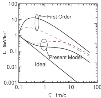
Now, we show our numerical results. To compare to pre-vious works, we ignore the bulk viscosity. In Fig. 1, we show the energy density ε obtained by solving Eq.(53) as function of proper time τ. As the initial condition, we set ε(τ0) =1 GeV/fm3,Π(τ0) =Ω(τ0) =0 at the initial proper timeτ0=0.1 fm/c. The first two lines from the top represents
0.1
1
10
100
τ
fm/c
0.001
0.01
0.1
1
10
100
ε
G
e
V
/f
m
3
Ideal
Present Model
First Order
FIG. 1: (Color online) The time evolution of the energy density. The dashed curves correspond to the calculations with the constant vis-cosity and relaxation time. The first two lines from the top represents the results of the LL. Next two lines shows the results of our theory. The last line is the result of ideal hydrodynamics.
the results of the LL. The next two lines show the results of our theory. The last line is the result of ideal hydrodynamics. For the solid lines, we calculated with the viscosity and relaxation time which depend on temperature. Initially, the effect of vis-cosity is small because of the memory effect, the behavior of our theory is similar to that of ideal hydrodynamics. After the time becomes larger than the relaxation time, the memory ef-fect is not efef-fective anymore and the behavior is similar to the result of the LL. As we have mentioned, the behavior of our theory is the same as the result obtained in Ref. [22] in this case. For the dashed lines, we calculated with the constant viscosity and relaxation time,η=η(ε0)andτR=τR(ε0). In this case, the viscosity is constant so that the heat production stays longer and has a smaller slope as a function of time as-ymptotically.
0.1
1
10
100
τ
fm/c
0.001
0.01
0.1
1
10
100
ε
G
e
V
/f
m
3
Ideal
Ideal Tµυ(τ 0)
First Order Same Tµν(τ
0) as the first order
FIG. 2: The time evolution of energy density with the different initial conditions from Fig. 1. The dashed and short dashed lines represent the result of the LL and our theory, respectively . For comparison, our result of Fig. 1 is shown, again (idealTµν(τ0)). The last line from
the top is the result of ideal hydrodynamics. In this case, the energy heat-up is observed even in our theory.
production can overcome the temperature decrease due to the expansion.
VII. SUMMARY AND CONCLUDING REMARKS
In this paper, we proposed an alternative approach to this question, different from the IS. We start from the physical analysis of the irreversible currents according to the Landau-Lifshitz theory. Then, the irreversible currents are given by in-tegral expressions which take into account the relaxation time. In this way, causality is recovered and at the same time a sim-ple physical structure of the LL is preserved. In our approach, only one additional parameter was introduced, the relaxation time,τR. The resulting equation of motion then becomes hy-perbolic and causality can be restored [5]. Naturally, causality depends on the choice of the values of the parameters includ-ing the relaxation time within the framework of this approach.
More specifically, we verified that the linearized equation of motion for small perturbations in the homogeneous, sta-tic background coincides with Hiscock-Lindblom [32–34] ex-cept for the coupling among the different irreversible currents. These couplings are not included in our theory considering the Curie principle. Of course the Curie principle is believed to be valid in the regime of the first order theory and in the sec-ond order regime these couplings might be present. However, the existence of the Curie principle may imply that these cou-plings are small compared with the direct terms.
The essential difference of our formalism from the IS is the expression for entropy production. In the IS, entropy pro-duction is required to be positive definite algebraically. Thus, the integral form like our formulation is not possible even ne-glecting some coupling terms. We relaxed this condition, that is, the positiveness of entropy production is required only for hydrodynamical motion with time scales longer than the re-laxation time. For extremely violent change of variables, the instantaneous entropy change for a hydrodynamic cell would not necessarily be positive definite.
We have applied our theory to the case of the one-dimensional scaling solution of Bjorken and obtained the analogous behavior of previous analysis. In this case we can prove explicitly the positiveness of entropy production. We showed the time evolution of the temperature. As expected, our theory gives the same result of Ref. [22], because the no-acceleration condition used in Ref. [22] is automatically satisfied in this model. Note that our theory is applicable to more general case where the acceleration is important.
The transport coefficients contained in relativistic dissipa-tive hydrodynamics should in principle be calculated from QCD. In the first order theory, it is known that the transports coefficients can be calculated by the Kubo formula. However, this formula does not gives the transport coefficients in the second order theory, as is shown in Ref. [27] explicitly and the corresponding corrections should be evaluated.
Our theory is particularly adequate to be applied to the hydro-code such as SPheRIO which is based on the La-grangian coordinate system [17, 18]. Implementation of the present theory to the full three-dimensional hydrodynamics is now in progress.
Authors are grateful for fruitful discussion with C. E. Aguiar, E.S. Fraga, T. Hirano and T. Hatsuda. T. Koide would like to thank David Jou for useful comments. This work was partially supported by FAPERJ, FAPESP, CNPq and CAPES.
[1] T. Kodama, T. Koide, G. S. Denicol, and Ph. Mota, hep-ph/0606161.
[2] D. Teaney, Phys. Rev. C68, 034913 (2003). [3] C. Eckart, Phys. Rev.58, 919 (1940).
[4] L. D. Landau and E. M. Lifshitz,Fluid Mechanics(Pergamon, New York, 1959).
[5] I. M¨uller, Living Rev. Rel.2, 1 (1999).
[6] D. Jou, J. Casas-V´azquez, and G. Lebon, Rep. Prog. Phys.51, 1105 (1988); Rep. Prog. Phys.62, 1035 (1999),
[7] I. M¨uller, Z. Phys.198, 329 (1967).
[8] W. Israel, Ann. Phys. (N.Y.)100, 310 (1976). [9] J. M. Stewart, Proc. Roy. Soc. A357, 59 (1977).
[10] W. Israel and J. M. Stewart, Ann. Phys. (N.Y.)118, 341 (1979). [11] H. Grad, Commun. Pure Appl. Math.2, 331 (1949).
[12] I. Liu, I. M¨uller, and T. R, Ann. Phys. (N.Y.)169, 191 (1986). [13] R. Geroch and L. L. Phys. Rev. D41, 1855(1990).
[16] E. Calzetta, Class. Quant. Grav.15, 653 (1998).
[17] C. E. Aguiar, T. Kodama, T. Osada, and Y. Hama, J. Phys. G
27, 75 (2001).
[18] Y. Hama, T. Kodama, and O. Socolowski, Braz. J. Phys.35, 24 (2005).
[19] A. Muronga, Phys. Rev. Lett. 88, 062302 (2002); ibid 89, 159901(E) (2002).
[20] A. Muronga, Phys. Rev. C69, 034903 (2004). [21] A. Muronga and D. H. Rischke, nucl-th/0407114.
[22] R. Baier, P. Romatschke, and U. A. Wiedemann, Phys. Rev. C
73, 064903 (2006).
[23] R. Baier, P. Romatschke, and U. A. Wiedemann, nucl-th/0604006.
[24] C. Cattaneo, Atti del Semin. Mat. e Fis. Univ. Modena 3, 3 (1948).
[25] P. M. Morse and H. Feshbach,Methods of Theoretical Physics, p. 865 (McGraw Hill, New York, 1953).
[26] T. Koide, G. Krein, and R. O. Ramos, Phys. Lett. B 636, 96 (2006).
[27] T. Koide, Phys. Rev. E72, 026135 (2005)
[28] M. A. Aziz and S. Gavin, Phys. Rev. C70, 034905 (2004). [29] Such a memory function was also used in the hydrodynamic
equations to take into account the time delay necessary to ther-malize the micro turbulences in a large scale system such as supernova explosion. See T.Kodama, R. Donangelo and M. Guidry, Int. J. Mod. Phys.C9, 745 (1998).
[30] T. Koide, G. S. Denicol, Ph. Mota, and T. Kodama, hep-ph/0909117.
[31] See, for example, T. Koide, J. Phys. G31, 1055 (2005). [32] W. A. Hiscock and L. Lindblom, Ann. Phys. (N.Y.)151, 466
(1983).
[33] W. A. Hiscock and L. Lindblom, Phys. Rev. D31, 725 (1985). [34] W. A. Hiscock and L. Lindblom, Phys. Rev. D35, 3723 (1987). [35] U. Seifert, Phys. Rev. Lett.95, 040602 (2005).