Bachelor of Science
Atlas-based semi-automatic segmentation of
Whole-Body Diffusion Weighted Imaging images:
Quantification of tumor burden
Dissertation submitted in partial fulfillment of the requirements for the degree of
Master of Science in Biomedical Engineering
Advisers: Nikolaos Papanikolaou, Principal Investigator, Champalimaud Foundation
Cristina João, Hematologist, Champalimaud Foundation, Auxiliarly Professor, NOVA Medical School
Examination Committee
Chairperson: Prof. Dr. Carla Maria Quintão Pereira
Imaging images: Quantification of tumor burden
Copyright © Sílvia Alexandra Dias Almeida, Faculty of Sciences and Technology, NOVA University Lisbon.
The Faculty of Sciences and Technology and the NOVA University Lisbon have the right, perpetual and without geographical boundaries, to file and publish this dissertation through printed copies reproduced on paper or on digital form, or by any other means known or that may be invented, and to disseminate through scientific repositories and admit its copying and distribution for non-commercial, educational or research purposes, as long as credit is given to the author and editor.
This document was created using the (pdf)LATEX processor, based in the “novathesis” template[1], developed at the Dep. Informática of FCT-NOVA [2].
It is with great pleasure and satisfaction that I finish this important step of my life. This journey would not be possible without the contribution of many people who helped me to fulfill my goals, whether professional or personal.
First, I would like to thank the Champalimaud Foundation, especially Professor Dr. António Parreira and Professor Dr. Celso Matos for having me welcomed in the institu-tion.
To my adviser Dr. Nikolaos Papanikolaou, for the motivation, availability, confidence and for the valuable teaching transmitted during our meetings. Thank you for the oppor-tunity to have worked on such a fascinating project.
To my adviser Professor Dr. Cristina João, for the contagious passion for science, dedication, kindness and critical mind whenever I presented you the results.
The work of scientific research is necessarily a teamwork, and, in this sense, I would like to thank Eng. João Santinha and Dr. Francisco Oliveira who worked with me in the development of this project. I fully appreciate all the support and the reception from the first day. Thank you for your critical minds, advice and for always encouraging me to explore different solutions and go beyond what was expected.
To Dr. Joana Ip, Dr. Maria Lisitskaya, Dr. João Lourenço and Dr. Aycan Uysal for your valuable segmentation work, explanations and clarifications about bone marrow involvement imaging.
To my college friends, with whom I shared moments of true happiness, joy, but also despair during these five years. The motto "Tudo se faz" has really brought us here, right? To my partner, thank you for all the love, but most importantly, the friendship. Thank you for the long conversations, for sharing our fears and accomplishments, for the support, stability and for growing side by side.
Cancer is a leading cause of death worldwide. Treatment strategies rely on accurate tumor staging and surveillance by imaging screening. Whole-body Diffusion Weighted Imaging (DWI) has high value to detect, characterize and quantify malignancies with irregular diffusion patterns, such as Multiple Myeloma (MM). However, the large volume of imag-ing data hinders the readimag-ing process. Manual delineation (segmentation) of tumor sites becomes a time-consuming process and lacks reproducibility. The lack of adequate tools in clinical practice leads radiologists to perform only a qualitative description of DWI im-ages and measure of the biggest lesion diameter, an inherently subjective process. Arising from this need, this dissertation aimed to develop an algorithm to improve the process of segmentation of lesions of MM DWI images, to allow accurately and rapidly tumor burden quantification, by validating against radiologist’s manual segmentation. Quantification of bone lesions (hyperintense on DWI) volume without considering normally hyperintense organs was made possible due to the development of an atlas-based and a smart lesion detector algorithm. The first allowed the removal of normal hyperintense organs from the images to be studied, using a suitable registration procedure. The second applied an outlier detector algorithm and compared voxel-by-voxel and connected-component approaches on different b-value images (directly acquired and computed), to delineate lesions. T1-weighted images were also used to improve lesion detection. The atlas-based algorithm revealed good alignments against the manual segmentation: Dice Similarity Coefficient (DSC) of 0.63±0.03 for male and 0.58±0.05 for female. Regarding lesion detec-tion, the connected-component approach applied to the directly acquired b-value image was the method that presented the greatest similarity to the gold standard. Although not yet overcoming the manual segmentation performance, these results are suggestive of the great potential of semi-automatic registration methods combined with quantitative algorithms to analyze DWI images, assisting radiologists while defining tumor burden. Staging, prognosis and response analysis in several pathologies may be facilitated.
O cancro é uma das principais causas de morte no mundo. As estratégias de tratamento dependem do estadiamento preciso e da vigilância por exames de imagem. A Imagem Pon-derada em Difusão de corpo inteiro (DWI) tem valor elevado para detetar, caracterizar e quantificar doenças com padrões de difusão irregulares, como o Mieloma Múltiplo (MM). No entanto, o volume elevado de imagens dificulta o processo de leitura. O delineamento manual (segmentação) dos tumores torna-se um processo demorado e carece de repro-dutibilidade. A falta de ferramentas adequadas na prática clínica leva os radiologistas a descreverem apenas qualitativamente as imagens de DWI e a medir o maior diâmetro da lesão, um processo inerentemente subjetivo. Decorrente desta necessidade, a presente dissertação teve como objetivo desenvolver um algoritmo para melhorar o processo de segmentação de lesões em imagens de DWI de doentes com MM, permitindo a quanti-ficação rápida e precisa da carga tumoral, comparando com a segmentação manual de radiologistas. A quantificação correta do volume de lesões ósseas, sem considerar órgãos normalmente hiperintensos, foi possível devido ao desenvolvimento de um algoritmo baseado num atlas e um detetor inteligente de lesões. A primeira permitiu a remoção dos órgãos hiperintensos normais das imagens a serem estudadas, utilizando um alinhamento adequado. O segundo aplicou um algoritmo de deteçãooutliere comparou as abordagens voxel-por-voxel e componentes-conectados em diferentesb-values. O algoritmo baseado no atlas revelou bons alinhamentos comparando com a segmentação manual: coeficiente de similaridade de Dice (DSC) de 0.63±0.03 para homens e 0.58±0.05 para mulheres. Em relação à deteção de lesões, a abordagem de componentes-conectados aplicada à imagem deb-valuediretamente adquirida foi o método que apresentou maior similaridade com os radiologistas. Apesar de ainda não superar o desempenho da segmentação manual, os re-sultados sugerem o potencial dos métodos de alinhamento semiautomáticos, combinados com algoritmos quantitativos para analisar imagens DWI. O estadiamento, prognóstico e análise de resposta poderão ser facilitados em várias patologias.
List of Figures xv
List of Tables xvii
Acronyms xix
1 Introduction 1
1.1 Context and Motivation. . . 1
1.2 Objectives and Dissertation Plan. . . 2
1.3 State-of-the-Art . . . 4
1.4 Dissertation Outputs . . . 7
2 Image Registration and Segmentation 9 2.1 Image Registration . . . 9
2.1.1 Transformation Model . . . 11
2.1.2 Similarity Measure . . . 12
2.1.3 Optimization Method. . . 14
2.1.4 Accuracy Assessment . . . 14
2.2 Image Segmentation. . . 15
2.2.1 Thresholding-based . . . 15
2.2.2 Edge-based. . . 17
2.2.3 Region-based . . . 18
2.2.4 Clustering-based . . . 18
2.2.5 Deformable models . . . 19
2.2.6 Atlas-based . . . 19
3 Magnetic Resonance Imaging and Diffusion 23 3.1 MRI Principles . . . 23
3.1.1 Image Contrast . . . 25
3.2 Diffusion Weighted Imaging . . . . 27
3.2.1 Pulsed Gradient Spin Echo. . . 30
3.2.2 Single Shot Echo Planar Imaging . . . 30
4.1 Multiple Myeloma . . . 33
4.2 Magnetic Resonance Imaging of Multiple Myeloma . . . 38
4.2.1 Bone marrow reconversion imaging. . . 38
5 Materials and Methods 41 5.1 Study Design and Population . . . 41
5.2 Imaging Protocol . . . 43
5.3 Image Processing Steps . . . 44
5.3.1 Atlas creation . . . 45
5.3.2 Smart Semi-automatic lesion detection in DWI images . . . 48
5.3.3 Automatic correspondence to T1w: more accurate lesion detection 50 5.4 Statistical analysis . . . 53
6 Results and Discussion 55 6.1 Atlas Creation . . . 55
6.2 Smart Lesion Segmentation. . . 64
6.2.1 Computed b-values . . . 64
6.2.2 Lesion Detection . . . 64
6.2.3 Similarity analysis: relation between manual and smart segmenta-tion . . . 92
7 Conclusions and Future Work 97 7.1 Limitations . . . 99
7.2 Future Perspectives . . . 99
Bibliography 101
A Appendix 1 113
1.1 Flowchart of a future MRI analysis, by the radiologist. . . 3
2.1 Typical registration methodology. . . 10
2.2 Representation of a distribution divided by quartiles. . . 17
2.3 Schematic representation of Multi-Atlas Segmentation steps. . . 20
3.1 T1 and T2 relaxation times. . . 25
3.2 T1-weighted tissues with different T1 relaxation times and T2-weighted tis-sues with different T2 relaxation times. . . . . 26
3.3 T2 decay curve. . . 26
3.4 Typical displacement distribution due to diffusion in a one-dimensional model. 27 3.5 PGSE sequence for DWI. . . 30
3.6 Loss of phase coherence of an individual diffusion spin. . . . . 30
3.7 SS-EPI sequence . . . 31
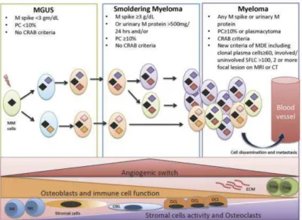
4.1 Biological evolution from MGUS to SMM to symptomatic MM and clinical criteria summary. . . 34
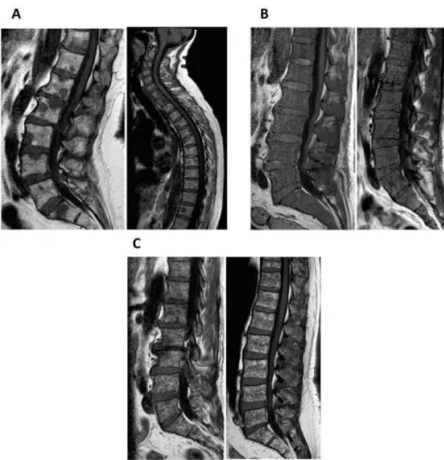
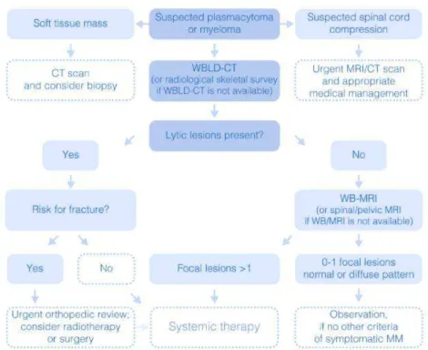
4.2 Appearances of focal, diffuse and variegated pattern on T1-weighted images. 36 4.3 Algorithm for imaging in MM. . . 37
4.4 Signal intensity change on high b-value and ADC images during the MM disease course: from MGUS, over SMM to MM. . . 39
5.1 Representative coronal slice of a WB-T1w and WB-DWI of the same patient. 45 5.2 First registration test. . . 46
5.3 Atlas building scheme. . . 48
5.4 Semi-automatic lesion detection in DWI scheme. . . 51
5.5 Example of a manually segmented label of a coronal slice of the Psoas muscle. 52 6.1 First mean male image, built with nine DWI male images. . . 56
6.2 First male template image, built with nine DWI images and using the previ-ously built mean image as the fixed image. . . 57
6.4 Male template image, built with 18 DWI images and using the first template image built with 18 images as the fixed image.. . . 58
6.5 Final male atlas, built with 42 DWI male images. . . 59
6.6 Final female atlas, built with 32 DWI male images. . . 59
6.7 Manually segmented hyperintense organs of the final male atlas and final female atlas. . . 60
6.8 DWI representative coronal image, manual and automatic segmentation of hyperintense organs. . . 61
6.9 Three different b-values applied to a male and female image. . . . . 65
6.10 Side-by-side comparison of manual and smart segmentation of Case 1 (male). 68
6.11 Side-by-side comparison of manual and smart segmentation of Case 14 (male). 70
6.12 Possible lesion on the iliac bone segmented by E3 and E4 on Case 8 (male) . 72
6.13 Side-by-side comparison of manual and smart segmentation of Case 11 (male). 74
6.14 Side-by-side comparison of manual and smart segmentation of Case 15 (male). 76
6.15 Several coronal representative slices of the legs of Case 16 (male). . . 77
6.16 Side-by-side comparison of manual and smart segmentation of Case 16 (male). 78
6.17 Representative coronal slices of the manual segmentation of Case 5 (male). . 79
6.18 Side-by-side comparison of manual and smart segmentation of Case 1 (female). 81
6.19 Side-by-side comparison of manual and smart segmentation of Case 12 (fe-male). . . 83
6.20 Side-by-side comparison of manual and smart segmentation of Case 13 (fe-male). . . 86
6.21 Side-by-side comparison of manual and smart segmentation of Case 1 (female). 87
6.22 Side-by-side comparison of manual and smart segmentation of Case 17 (fe-male). . . 88
6.23 Smart segmentation coronal results of Case 3 (female). . . 89
6.24 Side-by-side comparison of manual and smart segmentation of Case 4 (female). 90
6.25 Side-by-side comparison of manual and smart segmentation of Case 7 (female). 91
6.26 DSC distribution computed for the connected component approach using the highest b-value DWI image (800 or 1000 s/mm2) on male images. . . 93
6.27 DSC distribution computed for the connected component approach using the computed b-value DWI image (1500 s/mm2) on male images. . . 93
6.28 DSC distribution computed for the connected component approach using the highest b-value DWI image (800 or 1000 s/mm2) on female images. . . . . . 94
5.1 Demography of the female and male group. . . 42
5.2 Demography of the male and female atlases and male and female validation. 43
5.3 DWI acquisition parameters. . . 43
5.4 T1w acquisition parameters. . . 44
6.1 DSC, AHD and HD±standard deviation for each anatomical male label, seg-mented manually and automatically. . . 61
6.2 DSC, AHD and HD ± standard deviation for each anatomical femal label, segmented manually and automatically. . . 62
6.3 Average DSC, PPV, NPV, Sensitivity±standard deviation computed for the CC and VbV approaches using male images. . . 92
6.4 Average DSC, PPV, NPV, Sensitivity±standard deviation computed for the CC and VbV approaches using female images. . . 92
A.1 DSC, PPV, NPV, Sensitivity and averages computed for the SA and Experts, us-ing the CC approach on the highest b-value DWI images (800 or 1000 s/mm2) (male). . . 115
A.2 DSC, PPV, NPV, Sensitivity and averages computed for the SA and Experts, us-ing the CC approach on the highest b-value DWI images (800 or 1000 s/mm2)
(female). . . 116
A.3 DSC, PPV, NPV, Sensitivity and averages computed for the SA and Experts, using the CC approach on the computed b-value DWI images (1500 s/mm2)
(male). . . 117
A.4 DSC, PPV, NPV, Sensitivity and averages computed for the SA and Experts, using the CC approach on the computed b-value DWI images (1500 s/mm2)
(female). . . 118
A.5 DSC, PPV, NPV, Sensitivity and averages computed for the SA and Experts, using the VbV approach on the highest b-value DWI images (800 or 1000 s/mm2) (male).. . . 119
A.7 DSC, PPV, NPV, Sensitivity and averages computed for the SA and Experts, using the VbV approach on the computed b-value DWI images (1500 s/mm2)
(male). . . 121
A.8 DSC, PPV, NPV, Sensitivity and averages computed for the SA and Experts, using the VbV approach on the computed b-value DWI images (1500 s/mm2)
AB Atlas-based.
ADC Apparent Diffusion Coefficient. AHD Average HausdorffDistance.
CCC Champalimaud Clinical Centre.
cDWI computed Diffusion Weighted Imaging.
CT Computed Tomography.
DSC Dice Similarity Coefficient.
DWI Diffusion Weighted Imaging.
F18-FDG PET F18-Fluorodeoxyglucose Positron Emission Tomography.
FID Free Induction Decay.
HD HausdorffDistance.
IMWG International Myeloma Working Group.
LoG Laplacian of Gaussian.
MGUS Monoclonal Gammopathy of Unknown Significance.
MI Mutual Information.
MR Magnetic Resonance.
MRI Magnetic Resonance Imaging.
NCC Normalized Cross Correlation.
NIfTI Neuroimaging Informatics Technology Initiative.
NPV Negative Predictive Value.
PD Proton Density.
PET Positron Emission Tomography.
PGSE Pulsed Gradient Spin Echo.
PPV Positive Predictive Value.
RF Radiofrequency.
SA Smart Algorithm.
SMM Smoldering Multiple Myeloma.
SNR Signal to Noise.
SPECT Single-Photon Emission Computed Tomography.
SS-EPI Single Shot Echo Planar Imaging.
SSD Sum of Squared Differences.
STIR Short Tau Inversion Recovery.
TR Repetition Time.
WB Whole-Body.
WBLD-CT Whole Body Low Dose Computed Tomography.
C
h
a
p
t
e
1
I n t r o d u c t i o n
1.1 Context and Motivation
Accurate tumor staging and surveillance are critical when it comes to design optimal treatment strategies of malignant diseases. After confirming the diagnosis of a neoplastic disease, precise tumor localization and description of the degrees of organ infiltration are of paramount importance. Moreover, in order to assess the prognosis and to evaluate the response to therapy in a patient with a neoplastic disease, it is crucial to perform a precise identification and characterization of malignant lesions.
The anatomy of the human body has been subject of many studies and can be mapped in a non-invasive way by Magnetic Resonance Imaging (MRI),Computed Tomography (CT), digital mammography and other imaging modalities, facilitating diagnosis, staging of malignancies and treatment planning. In particular,MRIprovides anatomical images of the human body with a high spatial resolution and superb soft tissue contrast while there is no ionizing radiation exposure for the patient. Recent technological advance-ments inMRI made feasible the fact thatWhole-Body (WB) MRIcan be performed in the clinic in a reasonable examination times and without compromised image quality. Among these technological advancements are: utilization of more powerful and faster gradients, advances in hardware, use of a rolling platform-moving technology, phased array coils and parallel acquisition techniques [1].
expert, the reading process and manual delineation of the regions of interest becomes a painstakingly slow process, prone to error, hard to reproduce, time consuming with an increased risk of misinterpretation. Therefore, manual segmentation of large data sets is not a feasible solution [2]. Thence, nowadays, the gold standard for interpretation of
DWIis a qualitative description by an expert radiologist.
Fully-automatic and Semi-Automatic Segmentation algorithms have been developed over the years, in order to address this problem, speeding up and removing bias from the process. These approaches are decisive in terms of quantification and localization of lesion, diagnosis, study of the anatomical structure, treatment planning and computer--integrated surgery [3]. Semi-automatic methods are limited since they require several
user’s interventions, especially in the initialization step. Automatic identification and detection of structures in images using registration-based segmentation have been ac-cepted as a viable approach. The process involves a spatially normalized fitting of each image under study to the template image (or vice versa), facilitating posterior analysis [4]. Ideally, the template image is an average of the images under study, resulting in a better representation of the data available, and thus a better registration. Using just one image as the template would result in uncertainties and displacements in the registra-tion.Atlas-based (AB)segmentation approaches have also been used to fully automatic segmentation, which exploits already segmented template images (atlas images).
Despite the large number of studies about image segmentation and registration, these methods still need improvement regarding the difficulty of quantitative validation and adaptation to large data sets. DWI, in particular, has recently started to be studied for lesion detection using semi- or automatic segmentation and registration methods [2,5,
6, 7]. However, some of these studies have not been validated against expert manual segmentation. Therefore, there is a need for developing, improving and integrating novel registration and segmentation methods inDWI, in order to delineate specific regions pre-and post-treatment, assessing the response to therapy in neoplastic diseases.
1.2 Objectives and Dissertation Plan
The primary objective of the dissertation is the creation of a novelABsemi-automatic seg-mentation method for removal of hyperintense organs inWB-DWIimages. The secondary objective is to develop a smart segmentation algorithm of bone lesions inWB-DWIand to validate the algorithm in a cohort population of a group of neoplastic patients, diagnosed withMultiple Myeloma (MM), in different stages of the disease. It is also intended to validate by comparing the smart semi-automatic lesion detection to the expert’s manual segmentation. The main goal of the project, of which this dissertation is part, is to develop a smart segmentation tool (figure1.1) that, in the future, could be used by radiologists to assess tumor burden.
methods of accurately delineate tumor volume and further assessment of treatment re-sponse inWB-DWI. In chapter2are described some of the most common segmentation and registration techniques currently in use, and their specific advantages and disadvan-tages are highlighted. Afterwards, the relevant theoretical underpinnings of MRIand diffusion are explained. In chapter 4, the reader will be presented with an explanation about MM: symptoms, cause, resumed pathophysiology, and diagnosis. In the following chapter, the materials and methods used for imaging processing are presented. Then, the results and discussion will be presented. Lastly, are described the conclusions, limita-tions and future perspectives, which summarize the dissertation’s findings and suggest the next steps of this study.
1.3 State-of-the-Art
Medical image analysis emerged in the early 1990s, as a branch of Artificial Intelligence and Computer Science. In the beginning, mathematical methods that had gain traction in non-medical imaging problems, were applied to medical images [8]. In the following years, since the development of imaging techniques and digital imaging revolution, there was a need to enhance and delineate specific regions of the human body, in order to compare with other images or to quantify size or volume or to better study structures. Consequently, studies encompassing segmentation algorithms were rapidly developed.
Segmentation is one of the major problems in medical image analysis and consists in the process of subdividing a digital image into sets of pixels or voxels, tagging them with biological meaningful labels. For most applications, it remains as a manual task, where the expert sketches the contours slice by slice, using pointing devices like a mouse or a trackball. Thus, this approach is time consuming and prone to inaccuracies introduced by the user. Accuracy and precision are of great relevance to medical image segmentation, particularly to assess a prognosis and evaluate the response to therapy in neoplastic dis-eases. Therefore, specific segmentation algorithms are required in order to fulfill this gap in medical image analysis. Segmentation algorithms may differ from imaging modalities and different slices, since the appearances of a given organ may vary. Consequently, when designing an effective algorithm, it must be taken into account the imaging modality, structures to analyze, influence of noise and partial volume effects [9].
In addition to segmentation, registration is also of paramount importance in medical image analysis. It consists on the alignment of two or more images, allowing matching and comparison, fusion of different imaging modalities (e.g. MRI andCT) or to high-light structures of interest to facilitate further segmentation. The alignment is based on a transformation model, which defines the geometric transformation applied between images.
parts are object of studies: bones [14,15,16], heart [17], abdominal organs [18,19] and kidneys [20].
AB segmentation has become one of the most prominent approaches to semi- and fully-automatic segmentation. An atlas, in medical imaging, is a template image that represents all the images available for study. Usually, it is based on pairwise registration, where an image is selected as a reference and the other images are registered to it, one at a time, followed by an average of the result. Once the atlas is created, one can access the average location of human structures, such as bones, organs or tissues. Knowing the structures’ average position, segmentation can be done, either manual or automatic. Then, the segmented label can be transferred to the same physical space as a new image to be segmented, by applying the same transformation model used to register the images to the reference.
The usefulness ofAB segmentation has been shown in many studies [21, 22] and it is not restrained to an imaging modality. The introduction of multiple images as atlas - multi-atlas segmentation - can improve the representation of inter-subject variability,
compared to the use of a single atlas coupled with a deformation model [23].
Regarding WB-MRI, there have been developed some methods to fully automatic segment regions of the body. In order to assess measurements of the muscle volume, A. Karlssonet al[24] developed an automatic multi-atlas method for the quantification of total and regional skeletal muscle volume. This process involved segmentation of in-tensity-corrected water-fat separated image volumes, non-rigid registration of multiple atlas, muscle tissue classification and volume quantification. The validation showed high accuracy compared to manual segmentation. I. Lavdaset al[2] developed and evaluated three automatic methods of segmentation of organs and bones in WB-MRI, including a multi-atlas approach. This approach included an intensity-based image registration, with free-form deformations as the transformation model and correlation coefficient as the similarity measure. Although it did not improve the segmentation performance, com-pared to the gold standard manual segmentation, it is the foundation for the development of robust algorithms for the automatic detection and segmentation of lesions inWB-MRI
scans.
MMis a hematologic neoplasia characterized by clonal abnormal plasma cells in the bone marrow and/or in extramedullary sites, leading to hypercalcemia, renal insuffi -ciency, anemia and osteolytic lesions. Usually, tumor deposits occur on appendicular skeleton (proximal and long bones) but can also occur on the axial skeleton. The In-ternational Myeloma Working Group (IMWG) holds thatMRIis the gold standard for detection of bone marrow involvement inMM[25]. Normal, focal, diffuse, a combination of both focal and diffuse, and variegated are the typical patterns found onMRIofMM patients, when there is marrow involvement [26]. Diffuse pattern is often associated with advanced disease and worse prognosis [27,28].
Changes inADCvalue can be related to treatment response.DWIis commonly applied in oncologic imaging, helping to detect and characterize malignancies that show irregular diffusion behaviors.MMlesion’s patterns, for instance, have been recently evaluated by
ADCto help distinguish a diffuse from a normal pattern [29]. The results showed that
ADCs greater than 0.548x10⁻³mm2/s indicated 100% sensitivity and 98% specificity for the diagnosis of a diffuse pattern. Before extractingADCmetrics of total or partial lesion volume, tumor volume must be extracted inDWI. Traditional methods include manual delineation of the lesion, slice by slice. Yet, this is not applied in the common clinical practice: usually, the radiologist selects the larger sized lesion, measures its biggest diam-eter and extracts itsADC. This process can be considered very subjective when follow-up is performed: even if performed by the same radiologist, the diameter measured might not be the same. Plus, lesions are likely to not have a sphere-shape, which will translate into differences in diameter measures due varying positioning of the patient, between baseline and follow-up.
Adding to the fact that manual segmentation of lesions is a very difficult process, lacking high grades of agreement, it is estimated that radiologists have a 3-5% real-time day-to-day error rate and the retrospective error rate among radiologic studies is 30% [30]. To our knowledge, there is no study that compares the disagreement between lesion delineation inDWI-MRIby different radiologists, with different levels of experience.
Studies encompassing accurate tumor volume automatic delineation and further as-sessment of treatment response in WB-MRI are very few. Blackledge MD et al[7] de-veloped a semi-automatic segmentation algorithm ofWB-DWIusing a Markov random field model to infer tumor volume and associated globalADC. However, it still requires a lot of user interventions to define contrast between lesion and normal tissues and to define a threshold that covers the lesions. Also, it lacks on validating the segmentation algorithm, since they only evaluated based on responder/non-responder to treatment. Plus, the associated computational time is of the order of 30 minutes, which is considered long.
1.4 Dissertation Outputs
This dissertation has developed some output that was accepted for presentation in scien-tific events, which are worth mentioning:
Communication
• Almeida, D. S., Santinha, J., Oliveira, F., Papanikolaou, N., João, C., "Atlas-based semi-automatic segmentation of Diffusion Weighted Imaging", 3rd NOVA Biomedi-cal Engineering Workshop (NBEW), 9th May 2018, Caparica, Portugal.
C
h
a
p
t
e
2
I m a g e R e g i s t r a t i o n a n d S e g m e n t a t i o n
2.1 Image Registration
Image Registration, also known as image fusion, warping or matching, is a computa-tionally expensive task that involves deforming (using a suitable deformation model) an image until it is similar to another image. The purpose of this method is to find the opti-mal transformation that produces the best alignment of the structures of interest in the input images. The input images comprise a reference (fixed) and a moving image, that will be aligned with the reference one. Medical imaging, target recognition, cartography and computer vision are some of the main applications of this method [31].
Registration is a crucial step for medical image analysis since it is necessary in order to compare images from different sensors or modalities (multi-modal image registration), different viewpoints or even acquired at different times (serial image registration). Regis-tration can be applied intra-subject or inter-subject, when, e.g., the goal is to compare a certain characteristic in a given population.
Over the past decades, image registration has been the scope of several studies in medical image analysis [32], regarding fusion from anatomical images fromCT, fusion of functional images fromMRIandPositron Emission Tomography (PET),Single-Photon Emission Computed Tomography (SPECT)or functionalMRI. It can also be applied to diagnosis, staging, assessment of treatment response, detection of disease recurrence, surgery simulation, generation and comparison of atlas, radiotherapy, anatomic segmen-tation, comparison of images pre- and post-contrast injection and many others.
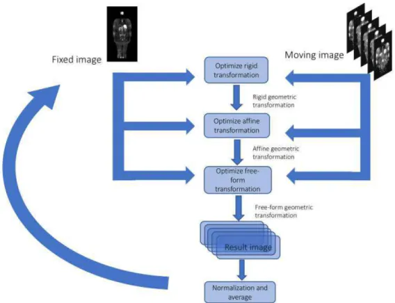
Typically, the process of image registration (figure2.1) involves the following compo-nents:
classes. The choice of the geometric transformation depends on the nature of the images to be registered.
• Asimilarity measureor alignment quality, which measures the degree of alignment between images. The methods for the alignment measure depend on the informa-tion contained in the image. Thus, measures can be obtained in terms of intensity intensitybased similarity measures or in terms of shapes, edges, landmarks
-feature-based similarity measures.
• Anoptimization method, which searches for the maximum or minimal value of the similarity measure adopted. The goal is to find a transformation that correctly registers the input images.
• Anaccuracy assessmentprotocol, which measures the performance of the registration protocol in terms of accuracy and reliability.
Figure 2.1: Typical registration methodology. The main idea is to search iteratively for the transformation model that optimizes the similarity measure, when applied to the moving image. The interpolator resamples the voxels/pixels of the moving image into the new coordinate system, defined by the search strategy (metric) found by the optimizer. Adapted from [33].
Usually, a simple pre-registration method is applied before the registration step, in order to obtain an initial solution. The moving image becomes closer to the fixed image in terms of the similarity measure, which allows a faster convergence of the optimizer and decreases the chance of an erroneous solution. The transformation model, similarity measure, optimization method and accuracy assessment protocol will be discussed in this chapter, as well as some of the applications in the clinic. Also, throughout this chapter,
The following content was mostly based on the literature review published by Oliveira & Tavares [4], B. Zitováet al[34] and Rueckert & Schnabel [35].
2.1.1 Transformation Model
The transformation model is given by equation2.1,
T: (x, y, z)→(x′, y′, z′) (2.1)
whose goal is to align each point in the moving image with the reference one.
Geometric transformations, defined by the transformation model, can be classified as non-deformable and deformable. Among non-deformable transformations, there is translation, rigid and affine transformations. Rigid transformation can be used when correspondence is achieved by simply rotation or translation of an image. It is defined in the 3D space by six degrees of freedom. Deformable transformations are applicable when correspondence between structures can only be achieved by stretching the image or other more complex transformation. Similarity (translation, rotation and uniform scaling), affine (translation, rotation, scaling and shear), projective and curved transformations are included in the deformable transformation class.
The transformation model chosen must be able to characterize the geometric transfor-mation between images, i.e., represent the transfortransfor-mations involved between them. For example, when registering rigid structures, as bones, of the same subject, there must be employed a non-deformable transformation. On the other hand, images that are affected, e.g., by respiratory motion must not be registered with a non-deformable transformation, since it does not represent the transformations required to align and deform the images. Plus, the model must be as simple as possible.
Both rigid and affine transformations can be characterized by a small number of pa-rameters, so they are considered simple. Rigid transformations are defined by three translational and three rotational parameters and can be applied in two situations. The first is for the registration of rigid structures, such as bones [36], [37]. The second is for pre-registration before a more complex transformation [38]. Affine transformations are defined by twelve parameters, represented by rotation, translation, scaling and shears. Thus, affine registration is more complete than rigid, since it enables corrections for scal-ing and shears. Rigid and affine transformations are suitable for registration of anatomical structures, like the brain and bones.
Usually, it is interpolated by the cubic B-spline, which allows very good alignments with high computational efficiency for a larger number of control points, since they are locally controlled. This means that when a control point is moved to a new position, only the point of the new position is affected, unlike global solutions (e.g. Thin-plate splines). Even though being locally controlled, B-splines can also be classified between a global registration and a local model, since they are controlled by a varying grid of controlling points. Thus, it is important to correct the global misregistrations before using free-form B-splines, for instance, with an affine transformation.
In guided transformations, the deformation is controlled by a physical model that takes into account the material properties, as the elasticity and fluid flow. This physical model treats the source image as a linear, elastic solid and is ruled by internal and exter-nal forces. Interexter-nal force is opposed to deformation of the material from its equilibrium shape, whereas external force acts on the moving image. Therefore, the deformation of the moving image stops when both forces reach an equilibrium. Local correlation mea-sure based on intensities, intensity differences or any gradient of a similarity measure mentioned in2.1.2can be used as an external force. Though, the linear elasticity assump-tion is only valid for small deformaassump-tions, so the elastic model is usually replaced by a viscous fluid model, also known as fluid-based algorithm. In this model, the registra-tion problem is addressed as a moregistra-tion problem, i.e. the content of an image is moved continually into the other, driven by the minimization of energy of the physical model adopted.
Finally, in order to preserve the topology of the structures represented in the images to be registered, the geometric transformation must be diffeomorphic. This means that it must be invertible and maps one differentiable manifold to another, so that both the function and its inverse are smooth.
2.1.2 Similarity Measure
After the selection of the geometric transformation between the images, the alignment between them must be measured. This measure of similarity is divided in two classes: the intensity- and the feature-based methods.
Intensity-based methods, also known as voxel-based methods, aims at measuring the degree of shared information between the images’ intensities. The most commonly used are based on intensity differences, intensity cross-correlation and information theory.
Intensity differences measurements are based on theSum of Squared Differences (SSD) (equation2.2), or their normalization, between intensities in the imagesΓAandΓB,
SSSD=
1
n X
((Γ
A(q)−ΓB(T(p)))2 (2.2)
to mono-modal applications. Ideally, if the images are correctly registered and, therefore, well aligned,SSSDis zero.
Intensity cross-correlation is a more general approach, based on the assumption that there is a linear relationship between the intensities of the images to be registered. It can be applied to some multi-modal tasks, but the majority is applied to mono-modal. The
Normalized Cross Correlation (NCC)is defined as follows in equation2.3,
SN CC= P
(Γ
A(q)−µA)(ΓB(T(p))−µB) p
(PΓ
A(q)−µA)2(PΓB(T(p))−µB)2
(2.3)
whereµAandµBare the voxel’s intensities average in the imagesΓAandΓB, respectively.
The larger theSN CCis, the better registered the image is.
In information theory, the images’content can be described as the Shannon-Wiener entropy,H(ΓA) andH(ΓB) of imagesΓAandΓB, computed from the joint probability
dis-tribution of the image voxel intensity. Equations2.4and2.5describe Shannon-Wiener entropy for both images,
H(ΓA) =−X a∈ΓA
p(a) logp(a) (2.4)
H(Γ B) =−
X
b∈ΓB
p(b) logp(b) (2.5)
wherep(a) andp(b) are the probabilities that a voxel in imagesΓ
A andΓBhas intensity a andb, respectively. Measurements of alignment can be obtained by the information content of the joint histogram obtained from the fixed and moving image, i.e., entropy of the joint histogram. The feature space of the image intensities can be seen as the joint probability distribution. The joint Shannon-Wiener entropy of the joint probability histogramH(ΓA,ΓB), of imagesΓAandΓB, may be defined by equation2.6,
H(Γ
A,ΓB) =− X
a∈ΓA X
b∈ΓB
p(a, b) logp(a, b) (2.6)
wherep(a, b) represents the joint probability that a voxel in the overlapping region of the imageΓ
A andΓBhasaandbas values, respectively. Information theory is mostly based
onMutual Information (MI), which can be defined as follows in equation2.7.
SMI(ΓA;ΓB) =H(ΓA) +H(ΓB)−H(ΓA,ΓB) (2.7)
MIis a measure of how well does one image explains the other image, so it is based on the supposition that there is a functional between the variables involved, e.g. the intensities. Therefore,MIis maximum when the images are correctly aligned. MIfails to consider relevant spatial information intrinsic to the original images since the computation is voxel by voxel, so only the relationships between corresponding individual voxels are considered.
is often computed using the sum of the distances between two fixed points, p andq
(equation2.8).
S=−X
i
kqi−f(pi)k2 (2.8)
Since points tend to be relatively sparse, surfaces of anatomical structures are commonly used when more dense features are required. Segmentation or landmark detection of the contours structures is a primary step in order to extract the features of the images. The resulting contours are represented as point sets, which can be registered by minimizing the distance between corresponding points of both sets. The correspondence between point sets needs to be known beforehand. One of the advantages of this method is that it can be applied to mono- and multi-modality registration. Since there is a need for feature extraction, some bias could be introduced if it is done manually, propagating the error to the registration process. As seen before, intensity-based methods have advantages over feature-based in this matter since does not require any feature extraction.
2.1.3 Optimization Method
Image registration problem can be assumed as an optimization problem, whose goal is to optimize an objective function. Frequently, the objective function is composed by two terms: the similarity measure between the images and a penalty term due to the geometric transformation. In the case of rigid or affine registration, the optimization algorithm is simply maximizing the similarity metric, since the last term plays no role. However, an affine registration can introduce unacceptable deformations. For non-rigid registration, the second term has a prominent role since it represents a prior knowledge about the expected transformation.
2.1.4 Accuracy Assessment
Validation of the registration algorithms are of great value in medical image analysis. Since the optimization problem relies on multiple adjustable parameters, the accuracy also depends on that choice.
There are several approaches to measure the accuracy of registration algorithms. As a first approach, the image similarity optimization could be used as a simple accuracy measure since in image registration the problem is defined as an optimization problem. Yet, it has little value in terms of geometry, so it is rarely used.
Points correspondence between images are an important measure of accuracy. Eu-clidean distance gives a physical value of the relation between correspondence points, so it is commonly used to assess accuracy.
2.2 Image Segmentation
Image segmentation is the process of extracting meaningful information from an image, separating it into several components. This method can be applied through an automatic or semi-automatic process. The difference between them is that semi-automatic segmen-tation requires user initialization and correction. Many image segmensegmen-tation methods have been applied to medical image analysis, facilitating the visualization and border detection of tissues and body organs.
Several image segmentation techniques exist, which can be divided in algorithms based on thresholding, edge-based, region-based, clustering, deformable models andAB. Similar to registration, segmentation methods also need to evaluate the performance of the algorithms, and so to assess the accuracy.
For instance,Dice Similarity Coefficient (DSC)is commonly used to evaluate the agree-ment between binary images, quantifying the matching between overlapping regions. This measure is frequently used to assess the degree of overlap of two segmentation. Equation 2.9 defines the Dice’s formula, whereA andB are two datasets. DSC equals twice the number of common elements of both groups divided by the sum of elements in each group. Thus,DSC=1 means that there is a complete overlap, whileDSC=0 means that there is not one single element in common between the datasets.
DSC =2∗ |A∩B|
|A+B| (2.9)
The following content was mostly based on the literature review published by L. K. Leeet al[39] and E. Neriet al[40].
2.2.1 Thresholding-based
Threshold-based segmentation methods are the simplest and straightforward methods, which are based on the assumption that images are formed from regions with different intensities. By analyzing the histogram of each images, if the intensity value is greater than some threshold, the corresponding pixels are targeted (foreground). If the value is lower than the threshold, the corresponding pixels are considered background. Equation
2.10represents the threshold-based method,
g(x, y) =
f oreground f(x, y)≥T background f(x, y)< T
(2.10)
value can be applied. This approach is considered global, since is based on the assumption that an object can be separated from the background using a threshold value. However, it fails when an image does not have a constant background, and only a region can be successfully segmented. In order to solve this problem, there can be applied local approaches. These approaches divide images into sub images and calculate the threshold for each one, and then the results are merged. Mean and standard deviation can be used to select the threshold value for each sub-image.
More sophisticated techniques have been developed, such as the Otsu’s method [41], which makes an initial guess of the thresholds and then maximizes the separation between different threshold classes in the data.
Thresholding can be combined with a connected-component analysis, which scans a binary image pixel-by-pixel from top to bottom, left to right, and identifies connected pixels, until a tissue type has been labelled. Then, a new threshold value is applied and the process is repeated for another tissue type.
2.2.1.1 Outlier Removal
Instead of defining a fixed numerical value for all images, above which segmentation occurs and the fact that some of theMRIsequences produce non-quantitative images, the value can be defined based on each image’s intensity distribution. For instance, when searching for specific regions in an image that stand out in terms of intensity (hypo or hyperintense), the image’s histogram can be calculated and the extremes (outliers) can be extracted.
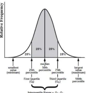
The Tukey’s fences [42] is one of the several methods to detect outliers [43,44,45]. If
Q1 andQ3 are the lower and upper quartiles, respectively, than the upper outlier range can be defined as a constant (k) multiplied by the interquartile range (difference between Q3 andQ1) plus Q3, and the lower outlier range as the difference between Q1 and k multiplied by the interquartile range. kis a non-negative constant. Tukeyet alsuggest usingk= 1.5 to define an outlier andk= 3 to define a range above that. However, when applied to imaging processing, this constant should be manipulated according to the size of the image and to highlight/remove.
Equations2.11and2.12define the outlier equations and figure2.2shows a distribu-tion divided by quartiles.
Upper outlier range≥Q3 +k(Q3−Q1) (2.11)
Figure 2.2: Representation of a distribution divided by quartiles. The first 25% is the first quartile (Q1), followed by the second quartile that represents the median (Q2) and the third quartile (Q3), corresponding to the 75% percentile. The interquartile range is defined as the distance between the third and first quartile. Adapted from [46]
2.2.2 Edge-based
Edge-based segmentation methods are based on the intensity variations presented in the borders of regions in an image. Sobel filters are gradient operators commonly applied to identify and extract borders.
The magnitude and orientation of an edge can be estimated by means of the Prewitt edge detector [47]. This operator calculates the gradient of the image intensity at each point, resulting in the direction of the largest possible increase from bright to darker values and the rate of change in that direction. Thus, the Prewitt edge detector provides information about how abruptly the image changes in a particular point, and thus how likely it could represent an edge, as well as its orientation.
Another example of edge-based methods are watershed algorithms. By combining image intensity with gradient information and using mathematical morphology opera-tions, they can divide images into homogenous regions. These homogenous regions are the pixels enclosed in the same watershed line, which are defined by the pixels with local maximum gradient magnitudes. Watersheds produce efficient segmentation due to the incorporation of diverse image information. However, these algorithms tend to suffer from over-segmentation, especially when the images are noisy or the desired objects have low signal-to-noise ratio appearances [9]. In medical image segmentation, this method is usually followed by a post-processing step to merge regions that were separated but belong to the same structure.
2.2.3 Region-based
Region-based segmentation algorithms consider the image to be analyzed as a homoge-nous region and aim to search for the pixels with similar feature values. Region Splitting and Merging and Region Growing are examples of region-based segmentation. The first, considers the image as a single region and then determines if the homogeneity criteria are satisfied. If not, the region is divided into smaller sub-regions. The process finishes when no further division is required. Then, the resulting sub-regions are compared and merged if they are similar.
Region growing algorithms incorporate the use of seed points, manually identified in the images. Then, a homogenous region is grown around the fixed seed points and neighboring pixels with similar intensities are iteractively added. The criteria adopted to decide if a pixel should or not be added and the connectivity used to determine neighbors depends on the algorithm adopted. The criteria behind the homogenous region growth can be threshold-based, i.e., select all the neighbors with intensity lower than or equal to the seed point’s intensity and above a threshold. The suitable threshold value can be obtained by a trial-and-error process or by the analysis of the image’s histogram.
2.2.4 Clustering-based
Clustering methods are unsupervised pattern recognition techniques that aim to divide and segment an image, without the use of training data. For this reason, clustering methods iteractively alternate between segmentation and characterization of the regions. Therefore, using only the data available, these methods can train themselves [3]. In this section, the most popular clustering algorithms will be explained, including K-means, fuzzy c-mean and Expectation Maximization. One of the advantages regarding these methods is that they consume less time, because do not use training data. However, these algorithms are sensitive to noise and intensity inhomogeneities since do not take into consideration the spatial information.
mean intensity for each class and the segmentation is done by classifying each pixel in the class with the closest mean. The mean of each class is iteratively updated as new pixels are added.
The fuzzy c-means algorithm generalizes the K-means algorithm, which tries to min-imize the intra-cluster variation through iterations. Instead of classifying a pixel into a fixed cluster, each pixel can potentially belong to multiple clusters, based on the proba-bility of belonging to each cluster. This algorithm provides a softer segmentation than the K-means.
The Expectation Maximization method iteractively calculates the maximum-likeli-hood estimation of the means and covariance. This algorithm is composed by two steps: calculation of the expectation of the likelihood and then its maximum. Although these methods are classified as unsupervised, they do need some initial parameters. The EM algorithm has demonstrated greater sensitivity to initialization, when compared to K--means or fuzzy cK--means algorithms [9], [48].
2.2.5 Deformable models
Based on the prior knowledge of geometry and physics, the deformable models are able to solve segmentation problems in a set of images over time and from different individ-uals. Level sets and active contours are examples of deformable models, which will be discussed in this section.
The level set is a numerical method used to account for the evolution of contours and surfaces. A curve is represented as the level set of a 2D scalar function, defined on the same domain as the image. The set of points that have the same function value defines the level set. The level set method evolves a curve by updating the level set function at fixed coordinates through time. Thus, in a typical approach, the contour is initialized by a user and then it is evolved until it fits the form of the anatomical structure intended [49].
Active contours, also called snakes, are based on the minimization of energy in splines. By defining an initial contour or a seed inside the object of interest, the active contour algorithm attempts to minimize the contour energy by moving the contour inside the target object.
2.2.6 Atlas-based
SimpleABsegmentation is based on a probabilistic atlas, where all the images avail-able are summarized. First, all images availavail-able are co-registered in a single atlas coor-dinate frame and statistics about the labels are pre-computed in the atlas space. The co-registered images are averaged to originate only a template image. To segment a new image, it is registered with the template and then it is segmented based on the segmenta-tion of the template.
Multi-atlas segmentation is an alternative strategy, in which different atlases can be used for the segmentation of the novel image, depending on the criteria. This method can be divided in four major steps: generation of atlases, registration, label propagation and label fusion (figure2.3).
Figure 2.3: Schematic representation of Multi-Atlas Segmentation steps.
The first step is the generation of atlases, i.e. the choice of which labeled training images yield the maximum performance when new data are segmented. This preselection can be done manually, by visual inspection or automatically. Accuracy of segmentation is affected by the proper choice of the training data, so low-quality images should be discarded. However, although it reduces the computational time, reducing the number of atlases can also affect segmentation.
After choosing the atlases, a match must be stablished between each atlas image with the target image - registration. Typically, it is computed between each atlas and the novel image, one independent intensity-based registration. Nevertheless, the choice of the registration approach depends on the data to be analyzed and can be constituted by the different modalities discussed in2.1.
Once the significant atlases are selected and spatial correspondence is stablished between each atlas and the novel image, the next step is to propagate the atlas labels to the novel image coordinates. This can be achieved by nearest neighbor interpolation, where a single label is transferred from the atlas to each image pixel/voxel, linear interpolation, signed distance maps or learning algorithms.
all atlases, to choose for the most frequent label at each location. However, it has the drawback of discarding the image intensity information. Alternatively, in weighted vot-ing, each atlas is associated with a weight. The higher the similarity between the target image with the atlas, the higher the correspondent weight.
C
h
a
p
t
e
3
M a g n e t i c R e s o n a n c e I m a g i n g a n d D i f f u s i o n
3.1 MRI Principles
This chapter was mostly based on the literature published by McRobbie & Donald W.et al[55].
MRI is a non-invasive diagnostic technique based on the atomic nuclei magnetic properties and the interaction of a nuclear spin with an external magnetic field,B0. MRI provides access to the anatomy and physiologic processes of the human body, with a high spatial resolution and excellent soft tissue contrast. Hydrogen is the most commonly used molecule due to high sensibility and abundance in human tissues. Hydrogen’s proton have an intrinsic magnetic moment,µ, and when subjected to a magnetic fieldB0
it rotates at a certain frequency, proportional to the field strength, which results in an angular momentum, the spin.
In the absence of an external magnetic field, the rotation of protons is random, and so the net value of the magnetization is null. On the other hand, when applying an external magnetic field, protons will align in the direction parallel or antiparallel to that of the field. Besides having a rotation movement around the magnetic field vector, the nuclear spin also rotates around that direction. The existence of two energy levels that protons can occupy inside the magnetic field is responsible for the two possible directions of alignment, due to the Zeeman effect. There is a division of the degenerated energy level, into a state of high energy (antiparallel) and low energy (parallel). Based on the Boltzmann distribution, the configuration of low energy is the preferred one. The difference of the protons’ distribution between the levels is the true contribution for the
MRIsignal, called longitudinal magnetizationM0.
with intensityB0is given by
w0=γB0 (3.1)
wherew0 is the Larmor frequency, γ is the gyromagnetic constant ration between the magnetic and the angular moment andB0is the magnitude of the magnetic field.
In order to acquire signal, there must be transitions between the higher and lower states of energy (antiparallel- and parallel), which must be induced by an external energy source, theRadiofrequency (RF)pulse. TheRFpulse must be applied perpendicular to
B0and at the Larmor frequency of the element in study so to induce resonance, which correspondes to the gap between the two levels of energy [56].
At rest, there is no transversal magnetization and the net magnetization vector only has the z component. When applying the RF pulse, the z component is reduced from its equilibrium value,M0, and the transversalxycomponent becomes non-zero. When this is done, the spins become synchronized and rotate at a given angle, which depends on the duration and intensity of the pulse. When theRFpulse is turned off, only the external magnetic field is on, so the spins relax into it again.
Considering the application of a 90◦ RF pulse, the longitudinal component M
z(0)
equals to zero and the transversal componentMxy(0) has its magnetization vector
arbi-trary. The magnetization at later times is given by the Bloch equations,
Mz(t) =M0(1−e−t/T1) (3.2)
Mxy(t) =Mxy(0)(e−t/T2) (3.3)
where T1 is the longitudinal relaxation time and T2 the transversal relaxation time. T1 is the relaxation along the B0 direction, also called spin-lattice relaxation since it corresponds to the re-establishment of the thermal equilibrium in the local environment. It is also defined by the time taken for 63% ofM0to recover after a 90◦RFpulse. T2 is the relaxation along the plane perpendicular toB0, or spin-spin relaxation, the time that transversal magnetizationMxy takes to fall 37% of its original value, determined based
on theRFpulse duration and intensity.
By plotting both curves on the same graph (figure 3.1) for a tissue with T1=5xT2 the differences of time scales are well distinguishable. Intrinsic magnetic design and differences in magnetic susceptibilities between different tissues cause spatial variations in the strength of the magnetic field, which influence the transversal relaxation. These interactions between spins and field inhomogeneities also contribute to T2, becoming a T2∗rate instead, shorter than T2.
TheMagnetic Resonance (MR)signal is obtained based on the Faraday’s Law of Induc-tion, wherein a changing magnetic field induces a voltage in a nearby conductor. In this case, the variation ofMxyis detected by a receiving coil, which induces the generation of
Figure 3.1: T1 and T2 relaxation times. Although occurring at the same time, T2 is faster than T1 [55].
3.1.1 Image Contrast
In order to emphasize certain tissues, MRI images can be weighted in three different parameters: T1, T2 andProton Density (PD). It is important to realize that these three parameters are properties of a given tissue and that an image can be obtained based on that certain property.
T1 weighted (T1w) images are obtained by setting a short time between two excitation
RF pulses, the Repetition Time (TR)(figure 3.2-1A). This allows less time for the net magnetization vector to recover, which means that long T1’s tissues do not have time to relax completely, weakening the signal. On the other hand, tissues with a short T1 (shorter thatTR) have time to relax completely, recovering their longitudinal magnetization prior to being flipped by the second 90◦ RF pulse. This results in a strong signal. On the contrary, selecting a longTRvalue reduces the T1 contrast between tissues, since they have time to recover their magnetization (figure3.2-1B).
To measure the signal, it is necessary to apply a 180◦ RF pulse after the 90◦ one, to realign the spins. After the first 90◦ RF pulse, FID occurs. Then, following the 180◦RF pulse surges a spin echo (figure3.3). The time between the 90◦ pulse and the echo is called echo time (Echo Time (TE)). If a series of 180◦ RFpulses is applied after the 90◦
RFpulse, T2 decay can be measured by the curve that passes by the maximum of theFID
and following echos.
T2 weighted (T2w) images are obtained by controlling theTE. If a shortTEis used, the transversal magnetization of the tissues does not have time to relax completely, thus re-sulting in a poor contrast (figure3.2-2A). However, by setting a longTEvalue, relaxation has time to occur for both long and short T2 tissues (figure3.2-2B) [57].
Figure 3.2: T1-weighted tissues with different T1 relaxation times (1) and T2-weighted tissues with different T2 relaxation times (2). A good contrast between T1w tissues can be obtained by setting a short TR, since the magnitudes of their longitudinal magnetization recovery will be different. A smaller difference between their recovered magnetization vectors is found when TR is long, since they have time to recover their longitudinal mag-netization, resulting in poor contrast between them. A good contrast between T2w tissues can be obtained by setting a long TE, allowing almost complete transverse magnetization recovery. By setting a short TE, there is almost no difference between the loss of transverse magnetization of the two different tissues. Adapted from [57].
Figure 3.3: T2 decay curve. After the 90◦ RF pulse, FID occurs. T2 decay is defined by the curve that passes the maximum of the FID and following echos, result of setting the 180◦RF pulses [58].
3.2 Di
ff
usion Weighted Imaging
Molecular diffusion, or Brownian motion, is the random movement of molecules in fluid (e.g. water) drove by thermal energy. Thus, in the three-dimensional space, the water molecules’ trajectory is not predictable. When restricted to a close space, the molecules’ trajectory is no longer random since the physical barriers restrain the natural process of diffusion. The displacement can be characterized by the diffusion constant,D, given by the Einstein’s equation,
D=R2
6t (3.4)
whereR2is the mean square displacement andtthe time of observation, at a constant temperature [60]. The idea behind Einstein’s formalism is based on the experience of measuring the individual displacement of a given numberNof labelled water molecules in water, after a given time interval∆. For each displacement distancer, the numbernof
water molecules that reached that distance are counted. Then, a histogram of the relative number of labelled molecules (n/N) versus displacement distance (r) is plotted. Figure
3.4 shows a typical displacement distribution of diffusion in a homogenous medium, described as having a Gaussian distribution.
Figure 3.4: Typical displacement distribution due to diffusion in a one-dimensional model. For each displacement distance r, there is a corresponding proportion of molecules (n/N) within a voxel that were displaced that distance at a given interval∆
(the duration of diffusion experiment). For example, the red line indicates that at a given distancer, a certain proportion of molecules traveled that given distance. The horizontal color bar also shows the same Gaussian distribution and is indicative of high (blue) and low (red) probability of displacement. Adapted from [61].
diffusion. This phenomenon is called anisotropic diffusion, since it is time and direction dependent [61].
Diffusion is measured by the ADC, which depends on the gradients and time of application. The term apparent is due to the impossibility of differentiating diffusion from other sources of water mobility in in vivo acquisitions.ADCcan take values from 0 toD, varying from absence of diffusion to be the only water motion phenomenon present, respectively.
DWIallows mapping of the diffusion process of molecules in tissues, non-invasively, generating images with high contrast between tissues and with a micro structural res-olution. Contrast between tissues in T1 and T2 weighted is given by changes in the relaxation time, while functional MRIlies on blood oxygen level dependency. On the contrary, contrast between tissues inDWIis given by the changes of the water diffusion, dependent on the temperature, in biological tissues, namely inter, intra and extracellular. Consequently, these functional changes are visible before identified alterations on the morphologic routine sequences.
DWIsignal,Si, can be described by equation3.5,
Si=S0e−bADCi (3.5)
whereiis the direction to which gradients were applied,S0is the signal intensity with no diffusion weighting,ADC
i is the apparent diffusion coefficient measured ini direction
andb-value (s/mm2) defines the sensitivity degree to diffusion phenomenon and deter-mines the strength and duration of the diffusion gradients. It can be defined by equation
3.6.
b=γ2G2δ2(∆−δ
3) (3.6)
Equation 3.6 shows the dependence of the gyromagnetic constantγ, amplitude of the diffusion gradient G (mT/m), the duration of each gradient δ (ms) and the time interval between gradient pairs∆(ms). Manipulating these parameters allows different weightings of diffusion.
In order to fit the exponential function to calculate theADCmap, one must measure at least two b-values. Multiple b-values can be used to calculate theADCmap, improving its accuracy. However, it increases the scanning time [62]. Usually, are chosen a b-value of 0 s/mm2and one of 1000 s/mm2 to supress normal background, depending on the organs studied. A b-value of zero results in a T2-weighted image, as an anatomical reference, where healthy tissues are more attenuated than lesions. The higher the b-value, the stronger the diffusion weighting and so the higher the contrast in pathogenic regions.