Non-linear analysis of composite structures with integrated piezoelectric sensors and actuators

QUANSE 2002 April 9-12 – 2002 University of Conceptión- Chile

NON-LINEAR ANALYSIS OF COMPOSITE STRUCTURES WITH INTEGRATED PIEZOELECTRIC SENSORS AND ACTUATORS

José M. Simões Moita*a, Cristóvão M. Mota Soaresb and Carlos A. Mota Soaresb

a

Universidade do Algarve, Escola Superior de Tecnologia Campus da Penha, 8000 Faro, Portugal

Email: jmoita@ualg.pt

b

IDMEC/IST–Instituto Superior Técnico Av. Rovisco Pais, 1049-001 Lisboa, Portugal

Keywords: Actuators and Sensors, Composite laminates.

Abstract

This paper deals with the geometrically non-linear analysis of thin plate/shell laminated structures with embedded integrated piezoelectric actuators or sensors layers and/or patches. The model is based on the Kirchhoff classical laminated theory and can be applied to plate and shell adaptive structures with arbitrary shape, general mechanical and electrical loadings. The finite element model is a nonconforming single layer triangular plate/shell element with 18 degrees of freedom for the generalized displacements and one electrical potential degree of freedom for each piezoelectric layer or patch. An updated Lagrangian formulation associated to Newton-Raphson technique is used to solve incrementally and iteratively the equilibrium equations.The model is applied in the solution of four illustrative cases, and the results are compared and discussed with alternative solutions when available.

__________________________________________________________________________________________ Introduction

In the recent years the study of smart structures has attracted significant researchers, due to their potential benefits in a wide range of applications, such as shape control, vibration suppression, noise attenuation and damage detection. The use of smart materials, such as piezoelectric materials, in the form of layers or patches embedded and/or surface bonded on laminated composite structures, can provide structures that combine the superior mechanical properties of composite materials and the capability to sense and adapt their static and dynamic response. The piezoelectric materials have the property to generate electrical charge under mechanical load or deformation, and the reverse, applying an electrical field to the material results in mechanical strains or stresses.

Many researchers considering mainly linear analysis have carried out the modelling of composite structures containing piezolaminated sensors and actuators using the finite element formulation. A pioneering work is due to Allik and Hughes [1], which analysed the interactions between electricity and elasticity by developing a tetrahedral finite element. Recent surveys can be found in Benjeddou [2], Senthil et al. [3] and Franco Correia et al. [4]. Recently Yi et al. [5] has developed a 3D finite element model to carry out the non-linear dynamic response of laminated adaptive structures using an updated Lagrangian formulation. A twenty-node solid element including electrical degrees of freedom is developed to analyse structures with piezoelectric sensors and actuators, and multipoint constraints for electrical degrees of freedom are used to simulate electrodes. The numerical results show that the deflection amplitude, vibration frequency and output voltage are significantly influenced by the large deformation of structures. A fully non-linear theory and corresponding model with integrated piezoelectric actuators and sensors accounting for geometric nonlinearities by using local stresses and strains measures and an exact co-ordinate transformation has been developed by Pai et al. [6] and applied to active control of plates. The model includes shear deformation of anisotropic laminated plates and assumes a higher order displacement field for in-plane displacements. Icardi et al. [7] also presents a mathematical model with detailed investigation of 3-D stress field of multilayered adaptive plates based on von Karman strain-displacement relations. Numerical results are presented for simply supported cross-ply plates with top and bottom actuators in cylindrical bending under distributed transverse loading.

In this paper we present a finite element model, based on classical plate theory, for static non-linear analysis of plate/shell structures with piezoelectric sensors and actuators. A simple and efficient three-node triangular piezolaminated plate/shell element with 18 generalised displacement degrees of freedom is used. The formulation introduces one electric potential degree of freedom for each piezoelectric layer of the finite element model. To show the applicability of the proposed model illustrative numerical examples are presented and compared with alternative solutions when available.

1 Displacement and Strain Fields

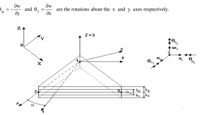
The classical Kirchhoff theory is considered. The displacement components (Figure 1) of a generic point in the laminated finite element local axes (x,y,z) are assumed to be of the form:

u(x,y,z)=u₀(x,y)− zθ_y v(x,y,z)=v₀(x,y)+ zθ_x (1) y) (x, w z) y, w(x, = ₀

y w x _∂ ∂ − = θ _and x w y _∂ ∂ =

θ are the rotations about the x and y axes respectively.

Figure 1. Three node triangular finite element with material (1,2,3) and geometric (x,y,z) coordinate

The present theory considers large displacements with small strains. The Green’s strains components associated with the displacement in equation (1) are given by:

                         

∂

∂

+

∂

∂

+

∂

∂

+

∂

∂θ

−

∂

∂

=

ε

0 2 2 0 2 0 y 0

x

w

x

v

x

u

2

1

x

z

x

u

xx               ∂ ∂       ∂ ∂       ∂ ∂ ∂ ∂θ ∂ ∂ ε 2 0 2 0 2 0 x 0 yy y w + y v + y v 2 1 + y z -y v = (2)

+

x

?

+

y

?

z

+

x

v

+

y

u

_{0 0} y _x xy          

∂

∂

∂

∂

∂

∂

∂

∂

=

ε

   

∂

∂

∂

∂

∂

∂

∂

∂

∂

∂

∂

∂

y

w

x

w

+

y

v

x

v

+

y

u

x

u

_{0 0 0 0 0 0}

3. Piezoelectric Laminates. Constitutive Equations.

In a piezoelectric material, the interaction between the mechanical and electrical fields is defined by Maxwell equations [8], l k kl k ij ijk kl ij ijkl

p

E

E

2

1

E

e

C

2

1

− = Φ

ε

ε

−

ε

(3) such that i E i D ; ij ij _∂ Φ ∂ − = ε ∂ Φ ∂ = σ (4)

__________________________________________________________________________________________ where E is the electric field vector, D the electric displacement vector, C the tensor of elasticity moduli,

ε

the strain tensor,

σ

the stress tensor, e the tensor of piezoelectric moduli, and p the tensor of dielectric constants, in material axes 1,2,3.

Substituting equations (3) into (4), the constitutive equations of a deformable piezoelectric medium are obtained. The linear piezoelectric constitutive equations coupling the elastic field and the electric field can be written as [9]

σ=Qε− eE

D=eT ε + pE (5)

where σ=

[

σ_xxσ_yyσ_xy

]

Tis the elastic stress vector and ε=

[

ε_xxε_yy γ_xy

]

Tthe elastic strain vector, Q the elastic constitutive matrix, e the piezoelectric stress coefficients matrix, E the electric field vector, D the electric displacement vector and p the dielectric matrix in the element local system (x,y,z) of the laminate.

The transformation of vectors and matrices from the orthogonal material axes system (1,2,3) to the local orthogonal system (x,y,z) of the laminate, in a state of plane stress, with transversal strains neglected, yields:           = 66 62 61 26 22 21 16 12 11 Q Q Q Q Q Q Q Q Q Q (6)           = 36 32 31 e 0 0 e 0 0 e 0 0 e (7)           = 33 22 21 12 11 p 0 0 0 p p 0 p p p (8)

where

Q

_ij are functions of ply angle α for the Kth layer, and are explicitly given in Reddy [9], and the piezoelectric and dielectric coefficients in the system (x,y,z) axes are related with the corresponding coefficients in the system (1,2,3) axes for the piezoelectric layers through [9]:

e₃₁=e₃₁cos2α+ e₃₂sen2α ; p₁₁=p₁₁cos2α+ p₂₂sen2α

e₃₂ =e₃₁sen2α+ e₃₂cos2α ; p₂₂ =p₁₁sen2α+ p₂₂cos2α (9) e₃₆ =(e₃₁-e₃₂)senαcosα ; p₁₂ =(p₁₁− p₂₂)senαcosα

p₃₃ =p₃₃

The electric field vector is the negative gradient of the electric potential

φ

, which is assumed to vary linearly in the thickness tk direction, i.e.

E=− ∇φ (10) E=

{

0 0 E_z

}

T (11) where E_z =−φ/t_k (12) Observing that [9]: e=Qd (13) with           = 36 32 31 d 0 0 d 0 0 d 0 0 d (14)

where

d

is the piezoelectric strain coefficient matrix in the local system (x,y,z) of the laminate, the equations (5) can also be written in the form:

(

dE

)

Q ε σ= −

D=(Qd)T ε + pE (15)

We can define the strain vector for electroelasticity in the form:

        − + = E eˆ NL L _ε ε (16)

where the mechanical strains are given by the sum of its linear and non-linear parts.

The linear part can be written in the form:

εL =ε_mL +zε_bL (17)

The constitutive equations (5) can be written in the synthetic form:

ε ε ˆεˆ E p e e Q D s sˆ NL L T =C         − +       =       = (18)

Integrating the stress vector σ through the laminate thickness, and substituting the vector σ by the first of equations (15), where the stresses are obtained as in linear analysis [10], one obtains the resultant forces and moments acting on the laminate:

__________________________________________________________________________________________

























′

′









































=

E

E

M

_bL

N

B

0

0

A

-D

B

B

A

=

~

mL

ε

ε

σ

₍₁₉₎

where the elements of the mechanical stiffness, for extensional, bending-extensional coupling and bending are given by:

∑

(

)

= N 1 k ij k k-1 ij = Q h -h A B = NQ

(

h -h

)

/2 1 k 2 1 -k 2 k ij ij ∑ = (i,j = 1,2,6) (20) D = NQ

(

h -h

)

/3 1 k 3 1 -k 3 k ij ij ∑ =

The elements of the piezoelectric stiffness are:

′ ∑

(

)

= P N 1 k im mj k k-1 ij = Q d h -h A (i,m,j = 1,2,6) (21) B = N Q_im d_mj

(

h_k2-h_k-12

)

/2 1 k ij P ∑ ′ =

where h is the laminate thickness and

h

_k,

k

_k−1 are the distances from the reference surface to the upper and lower surfaces of the Kth layer, N is the number of layers, and Npis the number of layers or patches with piezoelectric material.

Integrating the vector

D

through the thickness of piezoelectric patch or layer, and substituting the vector

D

by the second of equations (15), yields:

~

[ ]

A B -

[ ]{ }

A L m ' ε ε E D _L b ′ ′         ′ = (22) where N _ij

(

_{k k-1}

)

1 k ij = p h -h A P ∑ ′ ′ = (i,j = 1,2,3) (23)

4. Finite element formulation. 4.1 Updated Lagrangian formulation.

The virtual work principle is used in conjugation with an updated Lagrangian formulation to obtain the governing equations. A reference configuration is associated with time t, and the actualized

configuration is associated with the current time

t

+

∆

t

. The formulation of the element follows the development presented by Bathe [10]. The linearized equilibrium equations for a laminate finite element are:

( )

(

)

( )

ˆ ˆ dz dA (25) -= dA dz ˆ ˆ + dA dz ˆ ˆ ˆ N 1 = k _A h h e t k t T L k t e t t t N 1 = K e t A h h k t T NL k t A h h e t L k t k T L k t e t k 1 -k e t k 1 k e t k 1 -k ∑ ∫ ∫ δ ℜ ∑         ∫ ∫ δ ∫ ∫ δ ∆ + − σ ε σ ε ε ε C

Substituting equations (16) and (18), into equation (25), we can write:

(26)

dA

dz

ˆ

E

dA

dz

e

ˆ

0

e

+

dA

dz

E

p

E

N 1 = k _A h h e t k t T L k t e t t t e t A t k h 1 k h k t T NL k t N A t k h 1 -k h e t L k t k T T L k t e t k 1 -k 1 = k

e

e

Q

∑

∫ ∫

















−

δ

ℜ

=









∫ ∫

















δ

∑









∫ ∫

















−





























−

δ

∆ + −

σ

ε

σ

ε

ε

ε

By assuming that the loading is independent of the state of deformation, the term corresponding to the external virtual work is given by:

i i i 0 S t t 0 0 t t 0 i i i S 0 t t 0 V t t 0 t t S d Q V d q u F S d u T d u f 0 0 0

V

0 δφ ∑ + δφ ∫ + ∫ δφ + δ ∑ + ∫ δ + ∫ δ = ℜ ∆ + ∆ + ∆ + ∆ + ∆ + P V 0 (27)

where f is the body force, T the surface traction,

F

_i the concentrated force, q the body charge, Q the surface charge and

P

_i the point charge.

In the present work a three node triangular flat plate element is used to carry out geometrically non-linear analysis of general multilayered thin composite plate-shell type structures. As it is shown in Figure 1, the element has three nodes and six degrees of freedom per node, the displacements ui vi wi and rotations θ_xi,θ_yi,θ_zi. It requires the introduction of fictitious stiffness coefficients

K

θZ, corresponding to rotations

θ

z, which does not enter in the formulation in the local coordinate system

(x,y,z)[11]. The element local displacements u, v, w, are expressed in terms of nodal variables through shape functions given in terms of area co-ordinates Li [11]:

3 _i e 1 = i i = = N d Na d ∑ (28)

__________________________________________________________________________________________ e m m i 3 1 i m i m =∑B d =B a = ε (29) ε_b =∑Bb_id_i =Bb ae_b (30)

where the sub-matrices N ,_i B and m_i B are given by: _ib

[ ]

0 x x x 0 0 0 y y y 0 0 0 0 0 0 0 0 0 L 0 0 0 0 0 0 L i 3 i 2 i 1 i 3 i 2 i 1 i 3 i 2 i 1 i i i                     ∂ ∂ ∂ ∂ ∂ ∂ ∂ ∂ − ∂ ∂ − ∂ ∂ − = N N N N N N N N N N (31)

[ ]

                  ∂ ∂ ∂ ∂ ∂ ∂ ∂ ∂ = 0 0 0 0 x L y L 0 0 0 0 y L 0 0 0 0 0 0 x L i i i i m i B ;

[ ]

                    ∂ ∂ ∂ − ∂ ∂ ∂ − ∂ ∂ ∂ − ∂ ∂ − ∂ ∂ − ∂ ∂ − ∂ ∂ − ∂ ∂ − ∂ ∂ − = 0 y x N 2 y x N 2 y x N 2 0 0 0 y N y N y N 0 0 0 x N x N x N 0 0 i 3 2 i 2 2 i 1 2 2 i 3 2 2 i 2 2 2 i 1 2 2 i 3 2 2 i 2 2 2 i 1 2 b i B (32)

The electric field is given by

E=−Bφφ (33)

Substituting the last equations into equation (26), becomes:

dA dz D 0 0 a dA dz 0 0 0 0 0 a + dA dz a 0 0 p e e Q 0 0 a N 1 = k _A h h e t k t T mb T e t t t e t A h h _k t T nl T N 1 = K _A h h e t mb k T T mb T e t k 1 -k e t k 1 k e t k 1 -k ∑ ∫ ∫      σ               φ δ ℜ =     ∫ ∫      σ               δ ∑     ∫ ∫       φ               −               φ φ ∆ + φ φ −

δ

B B B B B B B (34)

To the first term of first member of equation (26) corresponds the linear stiffness matrix, which is defined by

_















=

φφ φ φ L L u L u L uu e L

K

K

K

K

K

_{∑ ∫ ∫}               −         = N _{φ φ} 1 = K _A h h e t mb k T T mb e t k 1 -k dA dz 0 0 p e e Q 0 0 B B B B (35) where we have: K N Bmb Q Bmb dz tdA 1 = K _A h h L uu T e t k 1 -k ∑ ∫ ∫ = ; K N Bmb e B dz tdA 1 = K _A h h L u T e t k 1 -k φ φ= ∑ ∫ ∫ (36) dA dz B e B K N T mb t 1 = K _A h h L u T e t k 1 -k φ ∑ ∫ ∫ = φ K B p B dz tdA N 1 = K _A h h L T e t k 1 -k φ φ φφ= ∑ ∫ ∫

The second term of the first member of equation (26), can be written in the form:

∑ ∫ ∫δ

( )

= = N 1 i e t A h h k t T NL k t dz dA e t k 1 -k σ ε _∫

( )

σ δ_ _ __ e t_A e t T ij u_s,i u_s,j dA 2 1 ˆ

(37)

where i,j =x,y and

u

_s

=

u

,

v

,

w

Considering the displacements on the reference surface only, the last equation can be written

_∫         δ σ e t_A e t ij u_s,i u_s,j dA 2 1 ˆ

=

_∫

{

[

δ + δ + δ

]

+ e t A . x , 0 x , 0 x , 0 x , 0 x , 0 x , 0 x u u v v w w N

2N_xy

[

u_0,x δu_0,y + v_0,x δv_0,y+ w_0,x δw_0,y

]

+ N_y

[

u_0,y δu_0,y+ v_0,yδv_0,y+ w_0,y δw_0,y

]

}

tdAe

(38) Thus the second term of the first member of equation (26), can be written in the form [12]:

∑ ∫ ∫ δ

( )

= = N 1 i e t A h h k t T NL k t dz dA e k 1 -k t σ ε ∫ δ

(

)

e t a a A e t e T e dA T G

τ

G (39) and the geometric stiffness matrix for the element is then given by:

0

0

0

K

K

K

K

K

_uu u u uu e

















=

















=

_σ σ φφ σ φ σ φ σ σ

K

(40) with K T tdA A uu e t G G

τ

∫ = σ ₍₄₁₎

__________________________________________________________________________________________ where the non-linear strain-displacement matrix G, and the matrix of actual membrane forces

τ

, are given by:

[ ]

                                ∂ ∂ ∂ ∂ ∂ ∂ ∂ ∂ ∂ ∂ ∂ ∂ ∂ ∂∂ ∂ ∂ ∂∂ ∂ 0 y N y N y N 0 0 0 x N x N x N 0 0 0 0 0 0 y L 0 0 0 0 0 x L 0 0 0 0 0 0 y L 0 0 0 0 0 x L = i 3 i 2 i 1 i 3 i 2 i 1 i i i i i G ;                     yy xy xy xx yy xy xy xx yy xy xy xx N N 0 0 0 0 N N 0 0 0 0 0 0 N N 0 0 0 0 N N 0 0 0 0 0 0 N N 0 0 0 0 N N = τ (42)

The first term of second member of equation (26), taken into accounting equation (28), and assuming the electric charge is zero, can be written as:

+∆ ℜ = ∫ δ + ∫δ + δ e o c T e 0 T A e e 0 S e T e e e 0 e T e T e t t _{a N p dA a N t dS a F}e ₍₄₃₎

where pe, te,Fe are the surface distributed, side distributed and concentrated force vectors. The external force vector is then defined

= _∫ + _∫ + e o_A 0 e e c e 0 S e T e e 0 e T e e ext p dA t dS F F N N (44)

To the second term of second member of equation (26), corresponds the internal force, which is defined by: ∫         ∫ =               =         = _{φ φ} e t T e t _A e t T mb A e t t T mb 2 int 1 int e int dA D~ s~ dA D~ s~ 0 0 F F B B B B F (45)

Equation (26) is valid for any virtual displacement field, δ ae and δφe. Considering the relations (35), (41), (44), (45), and introducing an iteration cycle, we have:

t_t++_∆∆_tt

(

K_Le + K_σe

) ( )

(k-1) ∆aˆe (k) = t+∆tF_exte − _tt₊+∆_∆t_t

( )

F_inte (k−1) (46) Numerical integration is used, with 3 Gauss points for matrices e

L

K

and Ke_σ and force vectors e

int e

ext and F

F . The element geometry, as well as stiffness matrices and external load vector are initially computed in the local coordinate system attached to the element. To solve general structures,

local - global transformations are needed [11]. After these transformations, the system incremental equations in referential X,Y,Z are:

_tt₊+_∆∆t_t

(

K_L+ K_σ

)

(k-1)

( )

∆qˆ(k) = t+∆tF_ext − t_t+_+∆∆_tt

( )

F_int (k−1) (47) where ∆qˆ=

{

∆q ∆φ( )S

}

T is the vector of incremental generalized displacements and electrical potentials, in the global coordinate system.

Assuming that piezoelectric sensors as well as actuators are bonded or embedded in the structure, the previous equation can be written in the following developed form:

(

)

















−





















φ

−









_φ

=













φ





































+

















+ + φφ + φ + + φφ φ φ + + 2 int 1 int ? t t ? t t (A) L(A) ? t t (A) L(A u ? t t mec ext ? t t (k) (S) 1) -(k s uu L(s) L(s) u L(s) u L uu ? t t ? t t

F

F

?

K

?

K

-

F

?

? q

0

0

0

K

K

K

K

K

) (48)

where A and S means actuator and sensor, respectively.

When we have actuators or sensors only, the system of equations (48) take the following forms, respectively:

(

[

]

)

{ }

{ }

{ }

1 int t t t t ) A ( L u t t mec ext t t ) k ( 1) -(k uu L uu t t t t K K q F K F ∆ + ∆ + φ ∆ + ∆ + σ ∆ + ∆ + + ∆ = − _ ∆φ(A)_− (49)

{ } { }

int t t t t ext t t ) k ( (S) 1) -(k uu L(S) ) S ( L u ) S ( L u L uu t t t t

F

F

q

0

0

0

K

K

K

K

K

_+∆ ∆ + ∆ + σ φφ φ φ ∆ + ∆ +

−

=













φ

∆

∆





































+





















(50) where     _∆φ = φ ∆ + A K F L(A) u t t act

is the force vector due to the voltage applied to the actuators.

The system of equations (50) can be decomposed, taking the form

[

L _uu

]

(k-1)

{ }

(k) t t

{ } { }

_extmec _tt _tt _int1 uu t t t t K K q F F ∆ + ∆ + ∆ + σ ∆ + ∆ + + ∆ = − (51)

{ }

[ ]

{ }

{ }

        − ∆         − = φ ∆ +₊∆_∆ φ ∆ + ∆ + − φφ ∆ + ∆ + 2 int t t t t ) k ( 1) -(k ) S ( L u t t t t 1 1) -(k L(S) t t t t ) k ( F q K K (52)

Once the boundary conditions are introduced in the usual way, the system equations (49) or the system equations (51) and (52) are solved incrementally and iteratively using the Newton-Raphson technique [13].

__________________________________________________________________________________________ 5. Numerical Applications

5.1 Linear analysis of a piezoelectric bimorph beam.

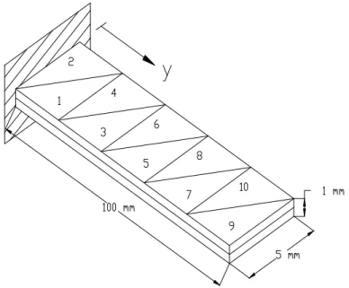
A linear analysis of a cantilevered piezoelectric bimorph beam, with two PVDF layers bonded together and polarized in opposite directions, with the dimensions indicated in Figure 2, is considered. The mechanical and piezoelectric properties of the PVDF are:

GPa, 2 2 E 1 E = = G₁₂=1GPA,ν₁₂ =0, e₃₁=e₃₂ =0.046C/m2,p₃₃ =1.062 x 10-10 F/m.

The top and bottom surfaces of the beam are subjected to an electric potential of 1V. The deflections in different locations of the beam, using a (5x2) element mesh, are presented in Table 1, which are compared with alternative solutions. The sensing voltage distribution of the bimorph beam for a prescribed tip deflection of 10 mm, is also analysed. The present predictions, and solutions obtained by other authors are shown in Table 2. The results are in good agreement with the alternative solutions.

Figure 2. Piezoelectric bimorph beam. Deflections x 10-7 m

Location y (mm) 20 40 60 80 100 Analytical solution

Suleman and Venkayya [12] 0.138 0.552 1.24 2.21 3.45 Q9-FSDT5P

Franco et al.[4] 0.138 0.552 1.24 2.11 3.45 FSDT4P

Suleman and Venkayya [12] 0.14 0.55 1.24 2.21 3.45

CPT Present Solution 0.137 0.550 1.240 2.210 3.45 Experimental

Suleman and Venkayya [12] - - - - 3.45 Table 1. Deflections produced by a unit voltage.

Sensed voltage (V)

Elements 1 and 2 3 and 4 5 and 6 7 and 8 9 and 10 Q9-FSDT5P Franco et al. [4] 290 226 161 97 32 FSDT4P Suleman e Venkayya [12] 290 - - - - Present Solution (CPT) 295 229 163 98 32 Table 2. Sensed voltage distribution for a tip deflection of 10 mm.

5.2 Non-linear analysis of a piezoelectric bimorph beam.

The sensing voltage on the elements 1 and 2 of the same cantilevered piezoelectric bimorph beam, is now analysed considering non-linear deformation. In Table 3 are shown the results for different load levels, where the load level µ=1.0 corresponds to the tip deflection of 10.0 mm in linear analysis. As expected from Table 3 a slightly decrease in the tip deflection is observed for the non-linear model, then resulting a lower voltage.

Linear analysis Non-linear analysis

Sensed voltage Tip deflection Sensed voltage Tip deflection Load level (V) (mm) (V) (mm) µ 0.2 59.00 2.00 59.00 2.00 0.4 118.00 4.00 117.76 3.99 0.6 177.00 6.00 176.42 5.98 0.8 236.00 8.00 234.91 7.94 1.0 295.00 10.00 293.08 9.89

Table 3. Sensed voltage on elements 1 and 2 for different load levels

5.3 Adaptive composite plate with surface bonded actuators

A simply-supported square (axa) laminated plate, with lamination sequence

[

p/45º/− 45º/45º/p

]

, where p represents the piezoelectric layers made of PXE-52, bonded on upper and lower surfaces, and the other layers are made of S-glass/epoxy. The plate is subjected to a uniform distributed load of 10 kN/m2 .

The material properties of S-glass/epoxy are :E₁=55GPa, E₂ =16 GPa, G₁₂ =7.6GPA, .

28 . 0

12 =

__________________________________________________________________________________________ GPa

24

G₁₂ = ,ν₁₂ =0.3, d₃₁=d₃₂ =−280x10-12m/V, d₃₃ =700 x 10-12 m/V, p₃₃ =3.45 x 10-8F/m .

The side dimension is a = 0.1 m and the thickness of the layers S-glass/epoxy and PXE-52 are 0.0004 m and 0.0002 m respectively.

The central deflection of the plate in linear analysis, for the uniform distributed load of 2

0 10kN/m

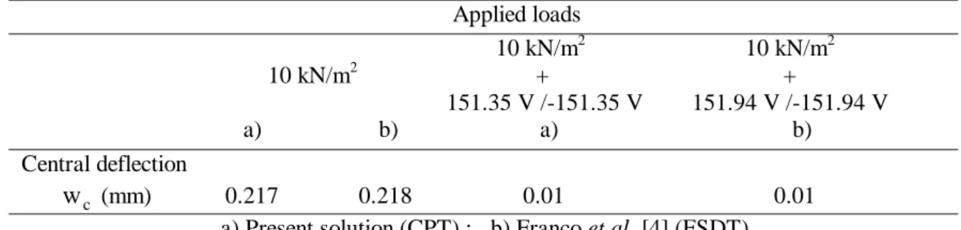
p = has the value of w=0.217 mm, using a (8x8) element mesh. Next it are applied voltages V of 151.35 V and –151.35 V on the lower and upper piezoelectric layers, in order to ₀ reduce the central deflection, produced by the mechanical load. The central deflection prediction of the present model shown in Table 4, are in a very good agreement with the alternative linear solution obtained by Franco et al [4], using a first order shear deformation piezolaminated 9 node plate element, with Lagrangian C0 shape functions to represent the generalized displacement field defined in the reference surface, and a constant potential degree of freedom for each piezoelectric layer within each element (Q9-FSDT5P model).

Applied loads 10 kN/m2 10 kN/m2 10 kN/m2 + + 151.35 V /-151.35 V 151.94 V /-151.94 V a) b) a) b) Central deflection

w

_c (mm) 0.217 0.218 0.01 0.01 a) Present solution (CPT) ; b) Franco et al. [4] (FSDT) Table 4. Central deflection for different load cases in linear analysis.

The same plate is also analysed taking into account non-linear deformations, for different load levels, defined by L=µ

(

p₀ + V₀

)

. Due to the lack of alternative comparing results, in Table 5 a convergence study is shown for non-linear central deflection at load level µ=3. It can be observed that for the meshes 8x8 and 10x10 the response is almost the same for the three cases of loading considered.

Mesh Total number of elements

Mechanical load Electric load Mechanical + Electric loads 2x2 16 0.501x10-3 -0.550x10-3 -0.531x10-5 4x4 32 0.608x10-3 -0.578x10-3 0.322x10-5 6x6 72 0.618x10-3 -0.589x10-3 0.332x10-5 8x8 128 0.621x10-3 -0.592x10-3 0.336x10-5 10x10 200 0.622x10-3 -0.593x10-3 0.337x10-5

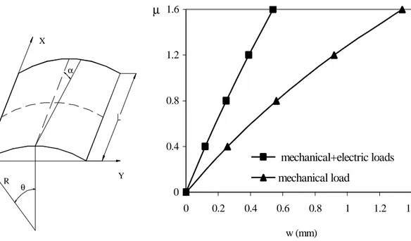
5.4 Adaptive laminated cylindrical panel with surface bonded actuators.

A laminated cylindrical panel, Figure 3, with lamination sequence

[

p/90º/0º/90º/p

]

, where p represents the piezoelectric layers made of PXE-52, bonded on upper and lower surfaces, and the other layers are made of S-glass/epoxy, is subjected to a concentrated central load. The panel is hinged in the straight edges, and free in the curved edges. The properties of two materials and the layers thickness are those indicated in previous application, and the geometry of the panel is: R=2540 mm, L=508 mm,

rad 1 . 0

=

θ . In Figure 4 are shown the load-displacement curves for two load cases, obtained with a (8x8) element mesh. The mechanical load is defined by Fext=µ F

0

ext with F 0

ext = 30 N, and the electric

load by V= µ V0 with V0=250 V. Other researchers can use the present predictions to validate

alternative non-linear piezolaminated shell models.

α X Y Z R θ 0 0.4 0.8 1.2 1.6 0 0.2 0.4 0.6 0.8 1 1.2 1.4 w (mm) µ mechanical+electric loads mechanical load

Figure 4. Cylindrical panel. Figure 5. Load-displacement curves.

6. Conclusions

A finite element model based on the Kirchhoff classical theory has been developed for the geometrically non-linear analysis of piezolaminated plates and shells, using update Lagrangian formulation. The model has been applied to linear and non-linear analyses of simple illustrative problems. The results obtained in linear analysis are compared with alternative models and an excellent agreement is achieved. The results also show that the transverse displacements are significantly influenced by the geometrically non-linear analysis. Due to the lack of available examples in the open literature, others can use the shown illustrative applications as a benchmark for comparing purposes.

Acknowledgments:

The authors thank the partial financial support of FCT/POCTI/FEDER, FCT-Proj. PRAXIS/P/EME/12028/1998, and Proj. 37559/EME/20001.

__________________________________________________________________________________________ References

1. H. Allik , T. Hughes, Finite element method for piezoelectric vibration. Int. J. Num. Meth. Engng., 2, (1970), 151-157.

2. A. Benjeddou, Advances in piezoelectric finite element modelling of adaptive structural elements: A survey. Computer and Structures, 76, (2000), 347-363.

3. V.G. Senthil, V.V. Varadan, V.K. Varadan, A review and critique of theories for piezoelectric laminates. Smart Material Structures, 9, (1999), 24-28.

4. V.M. Franco, M.A.A. Gomes, A. Suleman, C.M. Mota Soares, C.A. Mota Soares, Modelling and design of adaptive composite structures. Comp. Meth. Appl. Mech. Engineering, 185, (2000) 325-346.

5. S. Yi, S.F. Ling, M. Ying, Large deformations finite element analyses of composite structures integrated with piezoelectric sensors and actuators. Finite Elements in Analysis and Design, 35, (2000), 1-15.

6. P.F. Pai, A.H.Nayfeh, K. Oh, D.T. Mook , A refined non-linear model of composite plates with integrated piezoelectric actuators and sensors. I. J. Solids Structures, 30, (1993), 1603-1630. 7. U. Icardi, M.D. Sciuva, Large-deflection and stress analysis of multilayered plates with

induced-strain actuators. Smart Mater. Struct., 5, (1996), 140-164.

8. Penfield Jr, A.H.Hermann , Electrodynamics of moving media. Research Monograph Nº 40, The M.I.T. Press, Cambridge, Massachusetts, (1967).

9. J.N. Reddy, Mechanics of laminated composite plates. CRC Press, Boca Raton, New York, (1997).

10. K.J. Bathe, Finite element procedures in engineering analysis. Prentice-Hall Inc, Englewood Cliffs, New Jersey, USA, (1982).

11. O.C. Zienckiewicz , The finite element method in engineering Sciences, McGraw- Hill, 3 rd, London, (1977).

12. J.S. Moita, C.M. Mota Soares, C.A. Mota Soares, Buckling Behaviour of Laminated Composite Structures Using a Discrete Higher-Order Displacement Field. Composite Structures, 35, (1996), 75-92

13. M.A. Crisfield, Non-Linear Finite Element Analysis of Solids and Structures,Volume 1: Essentials, John Wiley and Sons, Chichester, UK, (1991).

14. A. Suleman, V.B. Venkayya, A simple finite element formulation for a laminated composite plate with piezoelectric layers. J. Intell. Mater. Sys. Structures, 6, (1995), 776-782.