Global Conservation Laws and Femtoscopy of Small Systems
Zbigniew Chaje¸cki1 and Mike Lisa1
1 Department of Physics, Ohio State University,
1040 Physics Research Building,
191 West Woodruff Ave, Columbus, OH 43210, USA
Received on 16 December, 2006
It is increasingly important to understand, in detail, two-pion correlations measured inp+pandd+A col-lisions. In particular, one wishes to understand the femtoscopic correlations, in order to compare to similar measurements in heavy ion collisions. However, in the low-multiplicity final states of these systems, global conservation laws generate significantN-body correlations which project onto the two-pion space in non-trivial ways and complicate the femtoscopic analysis. We discuss a model-independent formalism to calculate and account for these correlations in measurements.
Keywords: Proton collisions; Femtoscopy; Heavy ions; Pion correlations; RHIC; LHC
I. INTRODUCTION
The unique and distinguishing feature of heavy ions is their large (relative to the confinement scale) size and the possibil-ity to generatebulksystems which may be described in ther-modynamic terms, allowing to discuss the Equation of State of strongly-interactingmatter. The primary evidence for the creation of bulk matter at the highest energies is the existence of strong collective flow [1]. The dominant feature of flow are the correlations between space and momentum which it gen-erates; thus, momentum-only observables such aspT spectra and azimuthal anisotropies [2–5] represent only an indirect projection of the effect. Femtoscopic measurements access space as a function of particle momentum, thus providing the most direct probe of the most crucial feature of heavy ion col-lisions [c.f. e.g. 6]. In particular, flow is manifest by a negative correlation between the “HBT radius” and the transverse mass (mT) of the particles [7].
Clearly, then, a detailed understanding of femtoscopic mea-surements in heavy ion collisions is crucial to proving the ex-istence of, or probing the nature of, the bulk system gener-ated in the collision. It is in fact possible to quantitatively interpret both the femtoscopic and momentum-only observa-tions at RHIC in consistent, flow-dominated models of the system [e.g. 8]. All seems well.
However, two-pion femtoscopic measurements are also common in e++e− or p+p(p¯) collisions [9]. In these collisions, too, “HBT radii” are observed to fall with mT. Speculations of the physics behind this observation have included Heisenberg uncertainty-based arguments, string-breaking phenomena, and temperature gradients; an excellent overview may be found in [10]. Typically, however, one might not expect the system created in a p+pcollision to exhibit bulkbehavior similar to that from heavy ion collisions.
Quantitative comparisons between femtoscopic measure-ments inA+Aandp+psystems have been complicated be-cause techniques for event-mixing, frame definitions, and the like, have been different in the particle-physics and heavy-ion communities. As importantly, kinematic acceptance and col-lision energies are usually quite different. Recently, however, the STAR experiment has reported the first preliminary study
of directly-comparable femtoscopic measurements fromA+A andp+psystems [11] at the same√sNN, using the same de-tector, and with identical techniques. The results indicate that the femtoscopic probe of flow– falling “HBT radii” withmT– is essentiallyidentical in the small and large systems. This might signal an unexpected “universality” in the spatial sub-structure of hadronic and heavy ion collisions. Unravelling the physics behind this similarity might provide new insight into the dynamical space-time substructure ofbothhadronic and heavy ion collisions.
Before drawing strong physics conclusions from “HBT radii” coming from fits to the pion correlations measured in p+pcollisions, however, the measured correlation functions themselves must be understood in detail. The STAR data show clear non-femtoscopic correlations which must be dis-entangled from the femtoscopic ones [11]. Femtoscopic cor-relations are those which depend directly on the two-particle separation distribution [c.f. 6]. Non-femtoscopic correlations may arise from string or jet fragmentation, resonance decay, or global conservation laws.
In this work, we explore the projection ofN-body Energy and Momentum Conservation-Induced Correlations (EM-CICs) onto a two-particle relative momentum correlation function. In Section II we briefly discuss the harmonic rep-resentation of the correlations which best illustrates the effect. In Section III we discuss EMCICs generated by a Monte Carlo event generator containing only global conservation laws. A method to calculate analytically (but using distributions from the data) EMCICs is shown in Section IV. This provides an “experimentalist’s formula,” given in Section V, useful to disentangle EMCICs from the data, allowing a femtoscopic analysis of the correlation functions. We summarize in Sec-tion VI.
II. SPHERICAL HARMONIC DECOMPOSITION OF
CORRELATION FUNCTIONS
At asymptotically high relative momentum |~q| (or |~k∗|),
0.9 1.0 1.1 1.2 1.3 1.4
)
out
C(Q
STAR Preliminary
0.9 1.0 1.1 1.2 1.3 1.4
)
side
C(Q
experimental CF
fit
[GeV/c] o,s,l Q
0.0 0.1 0.2 0.3 0.4 0.5 0.6 0.9
1.0 1.1 1.2 1.3 1.4
)
long
C(Q
FIG. 1: (Color online) Preliminary STAR two-pion correlation func-tions [11] presented as 1D projecfunc-tions in the Bertsch-Pratt decompo-sition.
6]) must approach a constant value, usually normalized to unity, independent of the direction of~q. Preliminary STAR measurements [11] of small systems, Fig. 1, show clear non-femtoscopic correlations in addition. Also shown is a fit with the commonly Gaussian (with Coulomb suppression) func-tional form [6]. Clearly, the fit is a poor representation of the data. We stress, however, that it is not the (non-)Gaussian na-ture of the source at issue here;anysource function will lead to vanishing femtoscopic correlations at large|~q|and will thus contradict the data.
We further stress that the problem is not one of normaliza-tion. Shown in the Figure is the common representation of the 3-dimensional correlation function into three 1-dimensional axes [cf 6]. The projections, then, are not independent and cannot be independently normalized. The problem is that the value approached at large |~q| depends on the direction in~q space.
One-dimensional projections present a limited tool for ex-ploring detailed structure of the three-dimensional correlation function. The spherical harmonic decomposition (SHD) is a much more efficient representation of the data which usesall of the data to show the shape of the correlation function in 3D~qspace. There, the spherical harmonic coefficientsAl,m, which depend onQ≡ |~q|, are calculated as
Al,m(Q) =
∑
binsi
C(Q,cosθi,φi)· Yl,m(cosθi,φi)Fl,m
¡
cosθi,∆cosθ,∆φ¢, (1)
whereFl,mrepresents a numerical factor correcting for finite bin sizes∆cosθand∆φ; it turns out not to depend onφi. The anglesθandφare related to the Bertsch-Pratt Cartesian coor-dinate system through
qo=Qsinθcosφ, qs=Qsinθsinφ, ql=Qcosθ. (2)
0.0 0.2 0.4 0.6
0.9 1.0 1.1 1.2 1.3 1.4 1.5 1.6
| [GeV/c] Q |
00 RE A
peripheral d+Au @ 200 GeV
fit
STAR PRELIMINARY
: [0.15,0.60] GeV/c T
k
0.0 0.2 0.4 0.6
-0.04 -0.03 -0.02 -0.01 0.00 0.01
| [GeV/c] Q |
20 RE A
0.0 0.2 0.4 0.6
-0.04 -0.03 -0.02 -0.01 0.00 0.01
| [GeV/c] Q |
22 RE A
FIG. 2: (Color online) Preliminary STAR two-pion correlation func-tions [11] presented in the SHD representation.
See [12] for a complete discussion.
Preliminary STAR correlation functions in the SHD repre-sentation [11] are shown in Fig. 2. Coefficients forl≥4 are much less significant, compared to error bars; to good approx-imation, the non-femtoscopic behavior is quadrupole (l=2) in nature.
The presence of non-femtoscopic correlations is clear from the non-vanishing behavior ofAl6=0,m’s at largeQ. However, it is by no means clear that these contributions to the correlation function areconfinedto largeQ. Thus, one cannot attempt to interpret the low-Qregion only in terms of femtoscopic corre-lations, while parameterizing or ignoring the large-Qregion; see [13] for further discussion.
III. EMCICS GENERATED BY THEGENBODMONTE
CARLO GENERATOR
Non-femtoscopic correlations may arise from a variety of sources. Jets will clearly induce momentum-space correla-tions between its fragmentation products. While this cannot be discounted, the low momentum of the pions under consid-eration (pT∼0.2 GeV) puts us squarely in the region in which factorization breaks down and the jet interpretation becomes significantly murkier. We do not explore this possibility here. In the kinematic region under consideration, string fragmen-tation may play a role; this is an area for future study, though significant model-dependence will be present.
[GeV/c] x p -1.5 -1 -0.5 0 0.5 1 1.5 [GeV/c] y p -1.5 -1 -0.5 0 0.5 1 1.5 [GeV/c] z p -1.5 -1 -0.5 0 0.5 1 1.5
phase-space weight = 5.62509741e-36
FIG. 3: (Color online) A high-probability multiplicity-30 event calculated by GENBOD . Lines correspond to particle momenta px,py,pz.
[GeV/c] x p -1.5 -1 -0.5 0 0.5 1 1.5 [GeV/c] y p -1.5 -1 -0.5 0 0.5 1 1.5 [GeV/c] z p -1.5 -1 -0.5 0 0.5 1 1.5
phase-space weight = 3.78350585e-44
FIG. 4: (Color online) A low-probability multiplicity-30 event calcu-lated byGENBOD. Lines correspond to particle momentapx,py,pz.
Without doubt, one physical effect which mustbe at play is momentum and energy conservation. As global conserva-tion laws, these provide anN-body constraint on the event, which projects down onto 2-body spaces. The observed non-femtoscopic effects [11] become more and more significant as the multiplicity (N) of the event decreases, as expected from conservation laws. It is these EMCICs which we focus on here.
To clearly understand the role of EMCICs, we would like to have events in which there is no other physics involved be-sides the conservation laws. Such a tool has been provided almost 40 years ago in the form of the GENBOD computer program [see 14, for an excellent write-up of the method and physics] in the CERN library. Given a requested total mul-tiplicity (N), a list of masses (mi) of emitted particles, and a total amount of energy (Etot) to distribute among them,GEN -BODreturns an event of random momenta (four vectors pj), subject only to the condition of energy and momentum conser-vation. More importantly, it returns, for each event, a weight proportional to the probability that the event will actually
oc-| [GeV/c] Q |
0.0 0.2 0.4 0.6 0.8
0.85 0.90 0.95 1.00 1.05 00 RE A CF (GenBod)
order - all components st 1 full calculations | [GeV/c] Q |
0.0 0.2 0.4 0.6 0.8
-0.02 -0.01 0.00 0.01 0.02 20 RE A | [GeV/c] Q |
0.0 0.2 0.4 0.6 0.8
-0.02 -0.01 0.00 0.01 0.02 22 RE A component T order - P st 1
component z order - P st 1
order - E component st
1
| [GeV/c] Q |
0.0 0.2 0.4 0.6 0.8
-0.005 0.000 0.005 0.010 40 RE A | [GeV/c] Q |
0.0 0.2 0.4 0.6 0.8
-0.010 -0.005 0.000 0.005 42 RE A | [GeV/c] Q |
0.0 0.2 0.4 0.6 0.8
-0.006 -0.004 -0.002 0.000 0.002 0.004 0.006 44 RE A
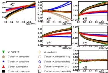
FIG. 5: (Color online) SHD coefficients for GENBOD -generated events consisting of 18 pions, as measured in the pair CMS frame. Green squares areAl,m’s from theGENBODevents. For discussion of
the other symbols, see Section IV.
| [GeV/c] Q |
0.0 0.2 0.4 0.6 0.8
0.85 0.90 0.95 1.00 1.05 00 RE A CF (GenBod)
order - all components st 1 full calculations | [GeV/c] Q |
0.0 0.2 0.4 0.6 0.8
-0.10 -0.08 -0.06 -0.04 -0.02 0.00 20 RE A | [GeV/c] Q |
0.0 0.2 0.4 0.6 0.8
-0.02 -0.01 0.00 0.01 0.02 22 RE A component T order - P st 1
component z order - P st 1
order - E component st
1
| [GeV/c] Q |
0.0 0.2 0.4 0.6 0.8
-0.01 0.00 0.01 0.02 0.03 40 RE A | [GeV/c] Q |
0.0 0.2 0.4 0.6 0.8
-0.04 -0.03 -0.02 -0.01 0.00 42 RE A | [GeV/c] Q |
0.0 0.2 0.4 0.6 0.8
-0.010 -0.005 0.000 0.005 44 RE A
FIG. 6: (Color online) Same as in Fig. 5, except only using pions with|η|<0.5 in the correlation function.
cur in nature. This weight is proportional to the phasespace integralRN
RN=
Z 4N
δ4
Ã
P− N
∑
j=1pj
! N
∏
i=1δ¡
p2i −m2i¢d4pi, (3)
whereP=³Etot,~0
´
| [GeV/c] Q |
0.0 0.2 0.4 0.6 0.8 0.90
0.95 1.00 1.05 1.10
00 RE
A
CF (GenBod)
component
T
order - P
st
1
component
z
order - P
st
1
order - E component
st
1
order - all components
st
1
full calculations
| [GeV/c] Q |
0.0 0.2 0.4 0.6 0.8 -0.02
-0.01 0.00 0.01 0.02
20 RE
A
| [GeV/c] Q |
0.0 0.2 0.4 0.6 0.8 -0.02
-0.01 0.00 0.01 0.02
22 RE
A
FIG. 7: (Color online) SHD coefficients for GENBOD -generated events consisting of 18 pions, as measured in the pair LCMS frame. Green squares areAl,m’s from theGENBODevents. For discussion of
the other symbols, see Section IV.
| [GeV/c] Q |
0.0 0.2 0.4 0.6 0.8 0.8
0.9 1.0 1.1
00 RE
A
CF (GenBod)
component
T
order - P
st
1
component
z
order - P
st
1
order - E component
st
1
order - all components
st
1
full calculations
| [GeV/c] Q |
0.0 0.2 0.4 0.6 0.8 -0.02
-0.01 0.00 0.01 0.02
20 RE
A
| [GeV/c] Q |
0.0 0.2 0.4 0.6 0.8 -0.02
-0.01 0.00 0.01 0.02
22 RE
A
FIG. 8: (Color online) Same as Fig. 7, but for 9-pion events.
expect, the “rounder” event is more likely, though one might be surprised by the factor of a hundred million between the probabilities.
Figures 5 and 6 show theAl,m’s calculated byGENBODfor 18-pion events without and with a selection of|η|<0.5, re-spectively. Note that this cut applies to the pions which are used in the analysis,notto the set of particles for which en-ergy and momentum is conserved; enen-ergy and momentum is always conserved for the full event. Clearly visible are signif-icant and nontrivialAl,m’s due only to EMCICs. We observe also that thel=4 coefficients are about an order of magnitude smaller than thel=2 ones; this is generically expected [cf 12]. Comparing the two figures, it is clear that kinematical se-lection has significant effect on the EMCIC effects. Also sig-nificant (but not shown) is whether one includes other species (say protons) into the mix of emitted particles.
Comparison of Figs. 7, 8 and 9 makes clear the multiplicity dependence of the EMCICs. As expected, lower multiplicity events show a greater effect. Also (not shown), increasing the
| [GeV/c] Q |
0.0 0.2 0.4 0.6 0.8 0.6
0.7 0.8 0.9 1.0 1.1
00 RE
A
CF (GenBod)
component
T
order - P
st
1
component
z
order - P
st
1
order - E component
st
1
order - all components
st
1
full calculations
| [GeV/c] Q |
0.0 0.2 0.4 0.6 0.8 -0.02
-0.01 0.00 0.01 0.02
20 RE
A
| [GeV/c] Q |
0.0 0.2 0.4 0.6 0.8 -0.02
-0.01 0.00 0.01 0.02
22 RE
A
FIG. 9: (Color online) Same as Fig. 7, but for 6-pion events.
amount of energy to be distributed among the particles, for fixed multiplicity, decreases EMCICs, as one expects.
Finally, we note that EMCICs can affect the correlation function even down to very lowQ, again reminding us that we cannot (responsibly) ignore these effects in a femtoscopic analysis.
IV. ANALYTIC CALCULATION OF EMCICS
Now then, EMCIC effects generated byGENBOD “resem-ble” the experimental data, but it is likely unwise to useGEN
-BODitself to correct the data for several reasons. Firstly, there is strong sensitivity to the (not completely measured) number and species-mix ofallparticles emitted in the event, includ-ing neutrinos and possible magnetic monopoles (or, less exoti-cally, particles escaping detector acceptance). Secondly, there is strong sensitivity to the energy “available” in the event; it is not obvious that this is√sNNof the collision. Clearly, EMCIC effects depend on the individual momenta~p1 and~p2 of the
particles entering the correlation function. This will depend on acceptance, efficiency, kinematic cuts and, to a degree, the underlying single-particle phasespace. (While correlation functions are insensitive to the single-particle phasespace, the correlations which they measure may, in fact, depend on this phasespace, due to physical effects.)
Thus, one would like to calculate EMCICs, based on the data itself. Here, we expand upon previous results [15–17] to write down correction factors which implement EMCICs onto multi-particle distributions.
A. Integral correction factors
Danielewicz [15], and later Borghini, Dinh and Olli-traut [16], considered EMCIC-type effects on two-particle azimuthal correlations (elliptic flow v2). They considered
re-cently considered momentum conservation effects on three-particle analyses of jet-like behavior [18].
As we shall see below, the conservation of energy generates effects of similar magnitude as does conservation of (three-) momentum. We deal only with on-shell particles, for which energy cannotbe treated as independent of the momentum (as, say, px would be largely independent of py). Thus, it is far from clear that we may simply take theD=4 case of ref-erence [17]. In fact, the distinction is significant in the final result, since inD=3⊕1, conservation of the final component couples into the first three, unlike theD=4 case [20].
Here, we remain in the case of interest –D=3 spatial di-mensions – and conserve 3-momentum~p. We implement en-ergy conservation and on-shell constraints a bit later.
We define [21]
f(~pi)≡ d3N
d~p3i (4)
as the single-particle momentum distribution unaffected by EMCICs. Then, the k−particle distribution (k less than the total multiplicityN)includingEMCICs is
fc(~p1, ...,~pk) =
Ã
k
∏
i=1f(~pi)
!
×
R³
∏Nj=k+1d3~pjf(~pj)
´
δ3¡
∑Ni=1~pi¢
R³
∏Nj=1d3~pjf(~pj)
´
δ3¡
∑Ni=1~pi¢ (5)
(Note the difference between numerator and denominator in the starting value of the index jon the product.)
In our case, we add in total energy conservation ∑Ei= √
s, which simply entails the replacement δ3¡
∑i~pNi=1i
¢
→
δ4¡
∑Ni=1pi−P¢ in Eq. 5, where P=
³√
s,~0´ is the total energy-momentum of the event, and p0
i =Ei=
q
~p2
i+m2i is the energy of the on-shell particle.
To apply the central limit theorem (below) to energy and momentum, we need to integrate independently over both. We begin by using the Lorentz-invariant distributions
˜
f(pi)≡2Ei d3N
d~p3i =2Eif(pi) (6)
and simply rewriting Eq. 5 as
˜
fc(p1, ...,pk) =
Ã
k
∏
i=1˜ f(pi)
!
×
R³
∏Nj=k+1
d3~p
j
Ej f˜(~pj)
´
δ4¡
∑Ni=1pi−P¢
R³
∏Nj=1
d3~p
j
Ej
˜ f(~pj)
´
δ4¡
∑Ni=1pi−P
¢
= Ã
k
∏
i=1˜ f(pi)
!
×
R³
∏Nj=k+1d4pjδ
³
p2j−m2j´f˜(pj)
´
δ4¡
∑Ni=1pi−P¢
R³
∏Nj=1d4pjδ
³
p2
j−m2j
´
˜ f(pj)
´
δ4¡
∑Ni=1pi−P¢
= Ã
k
∏
i=1˜ f(pi)
!
×
R³
∏Nj=k+1d4pjg(pj)
´
δ4¡
∑Ni=1pi−P
¢
R³
∏Nj=1d4pjg(pj)
´
δ4¡
∑Ni=1pi−P
¢ . (7)
Thus, we arrive at an integral over four independent variables, in which the integrand functiong(p)is “highly peaked” and with strong correlations in the 4-Dp−space.
According to Eq. 7, thek-body momentum distribution, in-cluding EMCICs, is the k-body distribution not affected by EMCICs – i.e. just an uncorrelated product of single-particle distributions – multiplied by a “correction factor” which en-forces the EMCIC. The numerator of this factor just demands that the remainingN−kon-shell particles are configured so as to conserve total energy and momentum, and the denominator just normalizes the distribution.
B. Application of the Central Limit Theorem
To arrive at a useful result, we wish to use the arguments of [15–17] to apply the central limit theorem (CLT) to Eq. 7. Those authors note that the distribution of a large numberM of uncorrelated momentaP′=∑Mi=1piis, by the Central Limit Theorem, a Gaussian distribution
FM¡P′¢ ≡
Z ÃM
∏
i=1d4pig(pi)
!
δ4
Ã
M
∑
i=1pi−P′
!
= 1
πσ2exp
Ã
−(P′)
2
2σ2
!
. (8)
Strictly speaking, it is not obvious that application of the CLT is valid in our case. The authors of [15–17] neglect any correlation inp-space of the single-particle distributiong(p). This means neglecting elliptic flow and any longitudinal de-pendence of thepTdistribution. These approximations should be fine, since the authors consider smallv2, and discuss effects
of transverse momentum only. In our cases, however, g(p)
so that for “large enough”N−k, we find [23] ˜
fc(p1, ...,pk) =
Ã
k
∏
i=1˜ f(pi)
!
×
µ N
N−k
¶2
·exp
"
−
3
∑
µ=0¡
∑ki=1(pi,µ− hpµi)¢
2
2(N−k)σ2
µ
#
(9)
where
σ2µ≡ hp2µi − hpµi2 (10) and
hp2µi ≡ Z
d pf˜(p)·p2µ. (11) Naturally, hp(µ=1,2,3)i=0. (In these equations, we now as-sume only one species of particles, so that no species label is needed for hp2µi. This is only for simplicity of notation here; results, including the “experimentalist’s formula” below, only become more cumbersome to write, but are similar oth-erwise.)
Note that even the single-particle momentum distribution is affected by EMCICs
˜
fc(pi) =f˜(pi)·
µ N
N−1
¶2
× (12)
exp
"
− 1
2(N−1) Ã
p2i,x hp2xi+
p2i,y hp2yi+
p2i,z hp2
zi
+(Ei− hEi) 2
hE2i − hEi2
!#
The k-particle correlation function is defined as the mea-sured (i.e. EMCIC-affected) k-particle yield divided by the product of the measured single-particle yields
C(p1, ...,pk)≡ ˜
fc(p1, ...,pk) ˜
fc(p1)···f˜c(pk)
= ¡ N
N−k
¢2
¡ N N−1
¢2k× (13)
exp
·
−1 2(N−k)
½
∑3µ=1
µ
(∑ki=1p2i,µ)
2
hp2µi
+(∑k1(Ei−hEi)) 2
hE2i−hEi2
¾¸
exp
·
−1 2(N−1)∑ki=1
½
∑3µ=1
p2i,µ
hp2µi+
(Ei−hEi)2 hE2i−hEi2
¾¸
An important point: EMCICs result from the constraint that the event’s energy-momentum is the same fixed number for all pairs in the event. This is true in the laboratory frame, but not in LCMS or pair rest frame. Thus, while one maybinthe correlation function in the frame of one’s choice, the momenta which appear on the right-hand-side of Eq. 13 must be in the laboratory system.
To first order in 1/N, the two-particle correlation function becomes
C(p1,p2) =1− (14)
1 N
µ
2~p1,T·~p2,T hp2Ti +
p1,z·p2,z
hp2
zi
+(E1− hEi) (E2− hEi)
hE2i − hEi2
where we have takenhp2xi=hp2yi=hp2Ti/2. In what follows, we shall refer to the first, second, and third terms within the
parentheses of Eq. 14 as the “pT term,” “pz term,” and “E term,” respectively.
If we knowN, hp2Ti, hpz2i, hE2i, and hEifrom the data, we can calculate EMCICs using Eq. 13. Better yet, ifN is large enough, then we can use Eq. 14. This is what is done in Figs. 5-8. The black circles, blue stars, and red triangles show the pT, pz andE terms, respectively, from the first-order ex-pansion (Eq. 14), while the open circles and orange inverted triangles represent the results of Eq. 14 and Eq. 13, respec-tively.
Several observations are in order. Firstly, each of the three terms in Eq. 14 produce non-trivial behavior of theAl,m’s, in-terfering with each other in interesting ways. We find also that thepzterm affectsA2,2; this was initially surprising sinceA2,2
quantifies the behavior of the correlation function in the “out-side” plane, while ˆzis the “long” direction in the Bertsch-Pratt system. Clearly, EMCICs projected onto a 2-particle space are non-trivial objects.
It is seen that the first-order expansion (Eq. 14) agrees well with the full expression (Eq. 13) well forN >∼10. Such multiplicities are relevant for thep+pmeasurements done at RHIC (especially recalling thatNincludes all particles, even unmeasured ones). We see also that the analytic calculations (open circles and inverted triangles) approximate the results of theGENBODsimulation (green squares), especially as the multiplicity and total energy of the event increases; increas-ing agreement for largeN andEtot is expected, given the ap-proximations leading to our analytic expressions. We observe also that the analytically-calculated expressions respond iden-tically to the kinematic cuts as does the simulation (c.f. Figs. 5 and 6).
Finally, the analytic calculations never reproduceexactly the simulations; we discuss this further in the next Section.
V. AN EXPERIMENTALIST’S FORMULA
Even for largeN and energy, the calculations do not ex-actly reproduce the EMCIC effects in the simulation. One reason for this may be found, in fact, in the definition of the average values (e.g. hp2zi) themselves. In Eq. 11, average quantities are calculated using the distribution ˜f(p), which is not affected by EMCICs. Naturally, the only measurable distribution available to the experimentalist (even whenGEN
-BODsimulations serve as the “experiment”) is ˜fc(p).
Thus, it appears the experimentalist cannot plug her data into the equations 10, 11 and 14 to fully calculate EMCICs. However, such an ambition would have been hopeless any-how. After all, even the total multiplicityN(again, including photons etc) is rarely fully measured. And finite kinematic acceptance (e.g. inη) will require extrapolation to calculate, e.g.hp2
zi.
un-derstand, we perform a fit. Let us rewrite Eq. 14 as
C(p1,p2) =1−M1· {~p1,T·~p2,T} −M2· {p1,z·p2,z} (15) −M3· {E1·E2}+M4· {E1+E2} −
M42 M3
.
where
M1≡
2
Nhp2Ti , M2≡ 1 Nhp2
zi
M3≡
1
N(hE2i − hEi2) , M4≡
hEi
N(hE2i − hEi2). (16)
The notation{X}in Eq. 15 highlights the fact thatX is a two-particle quantity which depends on p1andp2(or~q, etc):
{X}(~q). From a practical point of view,Xis averaged over the same~qbins as used for the correlation function. This involves nothing more than adding four more histograms to the several already being constructed by the experimentalist as she runs through all pairs in the data. The binned functions{X}then automatically reflect the same event and particle selection as the correlation function.
It is appropriate here to re-emphasize the point made in ref-erence to Eq. 13. The event’s total energy and momentum is a fixed quantity in a fixed (e.g. lab) frame; in particular, the mo-mentum in Eq. 13 is assumed~P=~0 – i.e. the collision-center-of-mass (CCM) frame is assumed. In a pair-dependent frame (e.g. pair center-of-mass PCM or longitudinally co-moving system LCMS), the event’s energy and momentum will de-pend on the pair. EMCICs, therefore, must be calculated with CCM momentum. Thus, in the function{p1,z·p2,z}(~q), p1,z andp2,zmust be calculated in the CCM frame, while the bin-ning variable~q should be in whatever frame one chooses to construct the correlation functionC.
The parametersMidefined in Eq. 16, on the other hand, are global and independent of p1 and p2. It is these which we
will use as fit parameters. The task is then fast and straight-forward; the EMCIC part of the correlation functionC(~q)is simply a weighted sum of four functions. Indeed, one may calculate coefficients as in Eq. 1 for the four new functions. For example
ApZ
l,m(Q)≡
∑
binsi
{p1,z·p2,z}(Q,cosθi,φi)· (17) Yl,m(cosθi,φi)Fl,m
¡
cosθi,∆cosθ,∆φ¢,
etc. Then, thanks to the linearity of Eq. 15 and the orthonor-mality ofYl,m’s, the measuredAl,m’s themselves are similarly just weighted sums of harmonics
Al,m(Q) =δl,0·¡1−M42/M3¢−M1·Alp,Tm(Q) (18)
−M2·Alp,Zm(Q)−M3·A(l,Em·E)(Q) +M4·Al(,Em+E)(Q).
Treating Eq. 18 as a fit, we have a few (say six, forl≤4) one-dimensional functions to fit with four adjustable weights. A first example of such a fit is shown in Fig. 10. Again
theGENBODsimulation is compared to the first-order form of
Eq. 15. The filled circles, stars and triangles show the “pT”
| [GeV/c] Q |
0.0 0.2 0.4 0.6 0.8 0.90
0.95 1.00 1.05
00 RE
A
CF (GenBod)
component
T
order - P
st
1
component
z
order - P
st
1
order - E component
st
1
order - all components
st
1
| [GeV/c] Q |
0.0 0.2 0.4 0.6 0.8 -0.03
-0.02 -0.01 0.00 0.01 0.02 0.03
20 RE
A
| [GeV/c] Q |
0.0 0.2 0.4 0.6 0.8 -0.02
-0.01 0.00 0.01 0.02
22 RE
A
full calculations component (FIT)
T
order - P
st
1
component (FIT)
z
order - P
st
1
order - E component (FIT)
st
1
order - all components (FIT)
st
1
| [GeV/c] Q |
0.0 0.2 0.4 0.6 0.8 -0.005
0.000 0.005 0.010
40 RE
A
| [GeV/c] Q |
0.0 0.2 0.4 0.6 0.8 -0.010
-0.005 0.000 0.005
42 RE
A
| [GeV/c] Q |
0.0 0.2 0.4 0.6 0.8 -0.006
-0.004 -0.002 0.000 0.002 0.004 0.006
44 RE
A
FIG. 10: (Color online)Al,m’s from 18-pion GENBOD -generated
events. Green inverted triangles (often underneath black squares) is the correlation function (measured in PRF) fromGENBOD. Filled brown circles, filled blue stars and filled red triangles show, respec-tively, the “pT,” “pz,” and “E” terms, defined in Eq. 14; black filled
squares show their sum. Open symbols of the same shape and color (identified as “FIT” in the legend) show corresponding terms, except with weights (see Eq. 16) adjusted to maximize agreement between the open black squares and the simulation.
(M1), “pz” (M2), and “E” (M3andM4) terms when the weights
(Eq. 16) are calculated directly from the events, as discussed in Section IV. Treating theMias adjustable parameters leads to a slightly different weighting of the terms, and a slightly better fit to the data.
Lest we forget, our original goal was not to understand EM-CICs per se, but to extract the femtoscopic information from measured two-particle correlations. Assuming that the only non-femtoscopic correlations are EMCICs, one may simply add the femtoscopic terms (e.g. Gaussian in(qo,qs,ql)space or whatever) to the fitting function in Eq. 15 or 18. Common femtoscopic fitting functions usually contain∼5 parameters (e.g. Rout) In the imaging technique [19], one assumes the separation distribution is described by a sum of splines (rather than, say, a Gaussian); here, too, there are usually 4-5 fit para-meters (spline weights). We have found that the number of fit parameters now must be doubled to account also for EMCICs. This is a non-trivial increase in analysis complexity. However, we keep in mind two points.
Secondly, while the non-femtoscopic EMCICs are not con-fined to the large-Qregion (an important point!), the femto-scopic correlations are confined to the small-Qregion. There-fore, one hopes that the addition of four new parameters to the fit of the correlation function will not render the fit overly unwieldy. While we can not expect complete block-diagonalization of the fit covariance matrix, one hopes that the Miare determined well enough at highQthat the femtoscopic fit parameters can be extracted at lowQ.
VI. SUMMARY
To truly claim an understanding of the bulk nature of matter at RHIC and the LHC, a detailed picture of the dynamically-generated geometric substructure of the system created in heavy ion collisions is needed. It is believed that this substruc-ture, and the matter itself, is dominated by strong collective flow. The most direct measure of this flow is a measurement of the space-momentum correlation (e.g.R(mT)) it generates. The physics of this large system, and the signals it generates, should be compared to the physics dominating p+p colli-sions, as is increasingly common in high-pT studies at RHIC. For the small systems, however, non-femtoscopic effects con-tribute significantly to the correlation function, clouding the extraction and interpretation of the femtoscopic ones.
EMCICs, correlations generated by kinematic conservation laws, are surely present and increasingly relevant as the event multiplicity is reduced. Using the codeGENBODto study
cor-relation functions solely driven by EMCICs, we found highly non-trivial structures strongly influenced by event characteris-tics (multiplicity and energy) and kinematic particle selection. We extended the work of Danielewicz and Ollitrault to in-clude four-momentum conservation and applied it to
corre-lation functions commonly used in femtoscopy. We found structures associated individually with the conservation of the four-momentum components, which interfere in nontrivial ways. Comparison of the analytic EMCIC calculations with
theGENBODsimulation gave confidence that the
approxima-tions (e.g. “large” multiplicityN) entering into the calculation were sufficiently valid, at least for multiplicities considered here. We further showed that the full EMCIC calculation can safely be replaced with a first-order expansion in 1/N.
Based on this first-order expansion, we developed a practi-cal, straight-forward “experimentalist’s formula” to generate histograms from the data which are later used in a generalized fit to the measured correlation function, including EMCICs and femtoscopic correlations.
The huge systematics of results and interest in femtoscopy in heavy ion collisions is renewing similar interest in the space-time signals fromp+pcollisions. Direct comparisons between the two systems are now possible at RHIC and have already produced intriguing (albeit preliminary) results. Very soon, p+p collisions will be measured in the LHC exper-iments, and the heavy ion experimentalists will be eager to apply their tools. The femtoscopic tool is one of the best in the box – so long as we keep it sufficiently calibrated with re-spect to non-femtoscopic effects increasingly relevant in small systems.
We would like to thank the organizers of this workshop– most especially the tireless Dr. Sandra Padula– for arranging a enjoyable gathering of experts in a very productive environ-ment. We wish to thank Drs. Mark Baker, Nicolas Borgh-ini, Ulrich Heinz, Adam Kisiel, Konstantin Mikhaylov, Jean-Yves Ollitrault, and Alexey Stavinsky for important sugges-tions and insightful discussions.
[1] Jean-Yves Ollitrault, Phys. Rev. D46, 229 (1992). [2] J. Adams et al.,nucl-ex/0501009
[3] K. Adcox et al.,nucl-ex/0410003. [4] B. B. Back et al.,nucl-ex/0410022. [5] I. Arsene et al.,nucl-ex/0410020.
[6] M.A. Lisa, S. Pratt, R. Soltz, and U. Wiedemann, Ann. Rev. Nucl. Part. Sci.55, 311 (2005).
[7] S. Pratt, Phys. Rev. Lett.53, 1219 (1984).
[8] F. Retiere and M.A. Lisa, Phys. Rev. C70, 044907 (2004). [9] Gideon Alexander, Rept. Prog. Phys.66, 481 (2003). [10] W. Kittel and E. A. De Wolf, p. 652 (Hackensack, USA: World
Scientific, 2005).
[11] Z. Chajecki, Nucl. Phys. A774, 599 (2006).
[12] Z. Chajecki, T. D. Gutierrez, M. A. Lisa, and M. Lopez-Noriega, nucl-ex/0505009.
[13] Z. Chajecki, AIP Conf. Proc.828, 566 (2006). [14] F. James, CERN-68-15.
[15] P. Danielewicz et al., Phys. Rev. C38, 120 (1988).
[16] Nicolas Borghini, Phuong Mai Dinh, and Jean-Yves Ollitrault,
Phys. Rev. C62, 034902 (2000).
[17] Nicolas Borghini, Eur. Phys. J. C30, 381 (2003). [18] Nicolas Borghini,nucl-th/0612093.
[19] D.A. Brown and P. Danielewicz, Phys. Lett. B398, 252 (1997). [20] As an example,pzconservation should not affect observables
in the transverse plane (e.g. elliptic flowv2), since pzis
inde-pendent ofpx,y. On the other hand, energy conservation, in the D=3⊕1 case, can in principle affectv2.
[21] Our use of symbols f and fc follows the convention used
in [16], which is significantly different – if unfortunately similar-looking – than that used in [17] and [18].
[22] The authors are grateful to U. Heinz for showing that on-shell conditions do not cause major complications in the extension to the formula to include energy conservation.
[23] In principle, also required for Eq. 9 ishEi2≫ hE2iso that
![FIG. 1: (Color online) Preliminary STAR two-pion correlation func- func-tions [11] presented as 1D projecfunc-tions in the Bertsch-Pratt decompo-sition.](https://thumb-eu.123doks.com/thumbv2/123dok_br/18982536.457573/2.892.489.825.75.347/color-online-preliminary-correlation-presented-projecfunc-bertsch-decompo.webp)