Catalysis with Competitive Reactions:
Static and Dynamical Critical Behavior
E. C. da Costa
N´ucleo de Pesquisa em Eliminac¸˜ao de Res´ıduos de Processos Produtivos, UNISUL
Campus da Grande Florian´opolis, Unidade II, 88130-000, SC, Brazil
and W. Figueiredo
Departamento de F´ısica, Universidade Federal de Santa Catarina
88040-900, Florian´opolis, SC, Brazil
Received on 11 April, 2003
We studied in this work a competitive reaction model between monomers on a catalyst. The catalyst is repre-sented by hypercubic lattices ind= 1,2and3dimensions. The model is described by the following reactions:
A+A→A2andA+B→AB, whereAandBare two monomers that arrive at the surface with probabilities
yA andyB, respectively. The model is studied in the adsorption controlled limit where the reaction rate is
infinitely larger than the adsorption rate. We employ site and pair mean-field approximations as well as static and dynamical Monte Carlo simulations. We show that, for alld, the model exhibits a continuous phase transi-tion between an active steady state and a B-absorbing state, when the parameteryAis varied through a critical
value. Monte Carlo simulations and finite-size scaling analysis near the critical point are used to determine the static critical exponentsβ,ν⊥and the dynamical critical exponentsν||,δ,ηandz. The results found for this competitive reaction model are in accordance with the conjecture of Grassberger, which states that any system undergoing a continuous phase transition from an active steady state to a single absorbing state, exhibits the same critical behavior of the directed percolation universality class.
I
Introduction
In the course of the last decade the statistical mechanics community has made great progress in the study of nonequi-librium phenomena. Until now, we do not have a complete theory accounting for the nonequilibrium systems. The fun-damental concept of a Gibbsian distribution of states in equi-librium has no counterpart in the nonequiequi-librium situation. This happens because many of these systems do not present even an hamiltonian function and, if it is possible to define an hamiltonian, the detailed balance would be violated.
Examples of recent problems on nonequilibrium pro-cesses include markets [1, 2], rain precipitation [3], sand-piles [4] and conserved contact process [5]. There is also a great interest in modeling interface growth [6, 7], traf-fic flow [8], temperature dependent catalytic reactions [9], etc. Nonequilibrium magnetic systems, with a well de-fined hamiltonian, have been also studied in the context of nonequilibrium processes [10, 11] as well.
For the equilibrium systems we can induce phase tran-sitions by changing some external parameters. Usually, the temperature is the selected control parameter to study phase transitions between equilibrium states. In the case of con-tinuous phase transitions, at the critical point, long range
correlations are established inside the system and a set of critical exponents can be defined to describe the critical be-havior of some thermodynamic properties. The renormal-ization group theory [12] is a well known theory that allows the calculation of these critical exponents.
We can also consider external constraints for the nonequilibrium systems that can drive the dynamical be-havior of the system. The nature of the external parame-ter depends on the nature of the system. For instance, in an epidemic model for the spread of a disease, the exter-nal parameter to be considered is the rate of change of the healthly individuals into unhealthly ones. In a catalytic reac-tion model, the external parameter can be the rate of change of the concentration of reactants. These, and many other ex-amples of nonequilibrium systems display dynamical phase transitions. A comprehensive survey on the dynamic phase transitions can be found in the books of Marro and Dickman [13] and Privman [14].
Recently, we have proposed a reaction model between monomers on a catalytic surface [18, 19] that can be viewed as a mixture of two other models: theA+A → A2 auto-catalytic reaction model and theA+B →AB monomer-monomer reaction model.
The monomer-monomer reaction model [20, 21] is the simplest catalytic reaction model, described by the reaction
A+B →AB, whereAandB are two monomers that ar-rive on a surface with probabilitiesyAandyB = 1−yA, respectively. This model was studied in the reaction con-trolled limit as well as in the adsorption concon-trolled limit. In both cases, ifyA > 0.5, the surface becomes saturated by monomersA, and the system always enters into an absorb-ing state. On the other hand, ifyA < 0.5, the absorbing state is one in which the lattice is completely covered by monomers of the typeB. However, ifyA= 0.5, the surface still saturates but with a much slower rate, and there is no preferred species to saturate the catalyst. The mapping onto the kinetic Ising model [22] showed that the time for the system to enter the absorbing state, at the particular value
yA = 0.5 and, in the reaction controlled limit, grows with the system size. Studies including monomers with different sizes [23], substrate viewed as a complete graph [24], in-troduction of a repulsive interaction between like monomers [25], the increase in the number of degrees of freedom for the reaction [26], are some examples of the research con-cerning the monomer-monomer reaction model carried out in the last decade.
On the other hand, the autocatalytic model [27] can be described by the reactionA+A→A2. This model was also considered by Aukrust, Browne and Webman [28], where they introduced a probability reaction between two adsorbed
Amonomers that occupy nearest neighbor sites on the lat-tice. Their model presents a continuous phase transition from a reactive steady state into an absorbing state, and the critical behavior of the model is in the same universal-ity class of the Directed Percolation. Through Monte Carlo simulations and finite size scaling analysis, they were able to find the static critical exponents of the model.
In our model, the catalyst was represented by a hyper-cubic lattice, and it is in contact with an infinite reservoir of monomersAandBin their gaseous phases. The monomers
A and B arrive at the surface with probabilities yA and
yB = 1−yA, respectively. These probabilities are related to the partial pressures of the gasesAandBinside the reser-voir. The model was investigated by effective field approxi-mations, as well as through static and dynamic Monte Carlo simulations ind = 1,2and3dimensions. The static criti-cal behavior exhibited by the model in two dimensions [18] put it in the same universality class of the Directed Perco-lation (DP). This was indeed expected, because the model presents a single continuous transition from a reactive sta-tionary state into an absorbing state, and the rate equations that describe the evolution of the system can be mapped onto those of the contact process. The dynamical critical behav-ior of the model in two dimensions [19] was also
investi-gated and we calculated the dynamical critical exponentsδ,
η andz, which control the asymptotic behavior of the sur-vival probability, the number of empty sites (the order pa-rameter of the model) and the mean square displacement of vacancies from the origin, respectively. For the calculation of the dynamical critical exponents, the simulations started with the lattice covered by monomers of the typeB, except in a central site, that is left empty. Thus, the configuration of the system in the beginning of the simulations is very close to the absorbing state. That study was made by employ-ing an epidemic analysis [29-31]. The dynamical critical exponents of the model are the same as those of Directed Percolation.
The DP universality class is the paradigm to describe the nonequilibrium phase transitions of a variety of mod-els. However, the experimental determination of the crit-ical exponents is too hard. In real systems, a perfect ab-sorbing state is not easily realized because there are always small fluctuations, for instance, due to thermal desorption of the elements. The presence of impurities, inactive sites and other inhomogeneities on the catalyst also difficult the measurements of the critical exponents. A full account on the possible experimental realizations of Direct Percolation can be found in the review work of Hinrichsen [32] and the references therein.
In the present work our main task is to extend the results found in two dimensions for the competitive reaction model to one and three dimensions. We present results obtained by employing mean field approximations, as well as static and dynamic Monte Carlo simulations. The model also exhibits continuous phase transition into an absorbing state, and the finite-size scaling arguments show that the model belongs to the same universality class of the Directed Percolation in all the dimensions considered in this work. This paper is organized as follows: in the next section we describe the model and we present the results obtained through the site and pair mean-field approximations in one, two, and three dimensions. In section III the model is studied by using static Monte Carlo simulations and finite-size scaling argu-ments. Section IV is dedicated to the study of the dynamical critical behavior of the model. In the last section we present our main conclusions.
II
Model and mean-field
approxima-tions
We consider a catalytic surface in contact with an infinite reservoir of monomers, labeled byAandB. The catalyst will be represented by a linear chain, as well as by square and cubic lattices. These monomers can be adsorbed onto the lattice, and they can react according to the following steps:
(ii) B(g)+v→B(a), (iii) A(a)+A(a)→A2(g),
(iv) A(a)+B(a)→AB(g).
The first two steps describe the adsorption of the species, and the other two, the possible reactions between adsorbed monomers that occupy nearest neighbor sites. Here, the(g)
and the(a)labels denote a monomer in the gaseous and in the adsorbed phases, respectively. The symbolvindicates a vacant site. The rules(i)−(iv)can also describe a lattice model for the birth and death of vacancies, resembling to the contact process. For instance, the processes(i)and(ii)
account for the annihilation of a vacancy due to the adsorp-tion of a particle, while the processes(iii)and(iv)give the birth of a vacancy due to the reaction step. For these reac-tions to occur, we need to have at least one vacant site, which is nearest neighbor of an adsorbed monomer. After the re-action, a pair of nearest-neighbor vacant sites is generated on the surface. In this way, we could resume the four steps above by a simple birth-death process for vacancies: v→ ∅ andv→2v. Then, we expect that our model is in the same universality class of the contact process [13], which belongs to the universality class of the DP.
It is convenient to introduce the following variables to describe the probabilities of the reactions:
ΠAA=
NA
NA+NB
; ΠAB =
NB
NA+NB
. (1)
If a monomer of the typeAadsorbs on an empty site sur-rounded byNAmonomers of the typeAandNBmonomers of the typeB, it will react with anyone of theAmonomers with the probabilityΠAA. In other words, ΠAA gives the probability of the occurrence of theA+Areaction in the presence ofBmonomers [33]. We must also introduce the quantityyA, which gives the probability that the next arriv-ing monomer to be of theAspecies. For theBmonomers
the probability isyB. These parameters are related to the ratio of the partial pressures of the gasesAandBinside the reservoir. Due to the fact that the partial pressures are nor-malized, we haveyA+yB = 1. Thus, the model has only a single independent parameter,yA. The dynamics of the model can be thought as a) the transport of monomers to the substrate, b) adsorption of the monomers onto the catalytic surface, c) surface reaction between adsorbed monomers, d) desorption of the products (the dimers) and e) transport of the products away the catalytic surface. Because we as-sumed an infinite reservoir of monomers, the steps a) and
e) occur instantaneously. In our modeling, we also consider
that the steps b) and d) are irreversible, and it is also sup-posed that the adsorbed monomers cannot diffuse on the lat-tice. We studied the model in the adsorption controlled limit, where the rate for the reactions is much larger than the rate for the adsorption.
A. Site approximation
In the site mean field approximation we neglect the cor-relations between neighboring sites, and we take all of them as being statistically independent. We consider that the sys-tem is translationally invariant. In this way, we define the densitiespi =Ni/Nas being the number of sites occupied by the speciesi divided by the total numberN of sites in the lattice. The labelistands for theAandBmonomers, as well as for the vacant (v) sites in the lattice. The densities are normalized,
pA+pB+pv= 1 . (2) Now, we need to calculate the transition probabilities de-scribing the steps(i)to(iv)presented before. In the table I we show the balance of the vacant sites.
Table I. Steps describing the processes(i)to(iv)in the site mean field approximation. 1.A+v→Aads. 2.A+v→A2↑+2v 3.A+v→AB↑+2v 4.B+v→Bads. 5.B+v→AB↑+2v
For instance, for the process 1, anA monomer in the gaseous phase arrives at an empty site and sticks there if all its neighboring sites are empty. On the other hand, for the process 2, anAmonomer in the gaseous phase arrives at an empty site and finds at least one A monomer adsorbed in its neighborhood. Then, they react instantaneously, forming the dimerA2, that immediately leaves the catalyst, and two new vacant sites are left on the surface. The time evolution of the densities is described by a set of differential equations that takes into account the five processes considered in the table I:
1. The rate for this process can be given by
T1=yApαv+1 , (3) whereαis the coordination number of the lattice.
2. To calculate the rate for this process we must consider all the possible configurations around the empty site where theAmonomer arrives. The table II lists all the combina-tions ofAandBmonomers.
T2=yApv α
X
j=1 α−j
X
i=0
Cα,jCα−j,ipjAp i
Bpαv−i−j
µ j
i+j
,
(4) whereCα,jstands for the combinatorics.
3. Analogously to the previous case, the rate for this process is
T3=yApv α
X
j=1 α−j
X
i=0
Cα,jCα−j,ipiAp j Bp
α−i−j v
µ j
i+j
.
(5) 4. In this case the rate is
T4=yBpv(pv+pB)α . (6)
Table II. Possible distributions ofAandB monomers around an empty site where there is anAmonomer arriving. The configurations listed in each column give the number ofA monomers and the possible distributions ofB monomers in a lattice of coordination numberα.
1A 0B 1B 2B .. .
(α−1)B
2A 0B 1B 2B .. .
(α−2)B
· · ·... (α−1)A
½ 0B
1B
¾
αA
5. The rate for this process can be given by
T5=yBpv[1−(pv+pB)α] . (7) With these rates we can write the gain and loss equations for the densities. For the density of the empty sites we have
dpv
dt = −T1+T2+T3−T4+T5
= yBpv−2yBpv(pv+pB)α+yApv(Sα−pαv) , (8) where
Sα= α
X
j=1 α−j
X
i=0
Cα,jCα−j,ipαv−i−j
³
piAp j B+p
j ApiB
´µ j
i+j
. (9)
After some algebraic manipulations we getSα= 1−pαv. The Eq. (8) can be written as
dpv
dt =pv[1−2yB(pB+pv)
α
−2yApαv] . (10)
This equation presents two stationary solutions,pv= 0and
1−2yB(pv+pB)α−2yApαv = 0 . (11) The solutionpv= 0indicates that the system evolves to aB-poisoned state, because theB−Breaction is forbidden. The other solution, Eq. (11), accounts for the reactive steady state, for whichpv 6= 0. Therefore, there must be a critical value of the parameteryA, for which the system changes from a reactive steady state to an absorbing one. Let us sup-pose that the system is poisoned, and it is in the vicinity of the critical valueyAc. By slightly changing the parameter
yA across the transition point, we allow for the appearance of some vacant sites. In this case, we can approximate Eq. (2) bypv+pB ≈1and the Eq. (11) furnishes
pv =
µ 1− 1
2yA
¶α1
, (12)
which gives the value1/2 for the critical value of the pa-rameteryA. For values ofyAthat are less than the critical, the system always evolves to a B-poisoned state whatever the initial condition we consider. The transition between the
B-poisoned state and the active steady state is described by a continuous phase transition, whose order parameter is the fraction of empty sites (pv), and the associated critical ex-ponentβis defined by the equation
pv∼(yA−yAc) β
. (13)
This mean-field approximation, at the site level, givesβ = 1/α.
B. Pair approximation
is the probability that a given site to be of typei, given that one of its nearest neighbors is of typej. We define the pair probabilitypij=pjP(i|j), that a randomly chosen nearest neighbor pair of sites are occupied by theiandjmonomers or they are vacant. The dynamics of the model is given by the rate of change of these pair probabilities, which are evaluated by counting the changes in the number of nearest neighbor pairs in a neighborhood of sites centered on, and including, the center pairi−j.
We need to consider only the pair probabilitiespvv,pvA,
pvB andpBBto describe this model, since the pairsi−j andj−i, although physically distinct, they contribute with the same weight to the equations of motion. The pair prob-abilities are related to the densities of monomers and to the fraction of vacant sites by the relationpj =Pipij. We may write the following relations
pA = pvA , (14)
pB = pvB+pBB , (15)
pv = pvA+pvB+pvv . (16)
Because of the relation given by Eq. (2) we can also write
pvv+pBB+ 2 (pvA+pvB) = 1 . (17) In this pair mean-field approximation we also suppose that these pair probabilities are all statistically independent and that the system is translationally invariant. The table III show all the possible transitions among the pairs.
Table III. Possible transitions among different configura-tions of pairs of nearest neighbors in the lattice.
From→ To↓
v−v v−A v−B B−B
v−v × T3 T4 ×
v−A T1 × × ×
v−B T2 × × T6
B−B × × T5 ×
For instance, the transitionT1means that the central pair is in the configurationv−v(both sites are empty) and there is anAmonomer arriving at the right site of the central pair
v−v, changing its configuration tov−A. The transition probability for this event is the same as that for the transi-tionv −v → A−v, since the pairsA−v andv−A
occur with the same probability. To calculate the transition probabilities we proceed in a manner similar to that used in the site mean-field approximation, but now they are more involved. Examples of the application of this pair approx-imation can be found in the references [34] and [35]. In particular, in the appendix B of the reference [34], a detailed description of the method used here is given, with emphasis to theN O+CO reaction model. The reaction probabil-ityΠAAwas defined as being the probability of an arriving
Amonomer to react with anyone of its nearest neighborA
on the lattice, in the presence of theB monomers. Now, it must be replaced by the probability of reacting with another selectedAmonomer, in the presence of theB monomers. Then,πAA= ΠAA/NA= ΠAB/NB = 1/(NA+NB). In this case,πAA=πAB, and the reaction probabilities are the same. Thus, the transition probability for the processT1is very simple and it is given by
T1=yApvv
µp
vv
pv
¶α−1
, (18)
while, for the process T3, the calculation is more in-volved. In this case, we have to consider two possible paths: monomerA(B)arriving at the vacant site of the central pair or arriving in a nearest neighbor site of theAmonomer of the central pair. In each case, all the possible distributions of
AandBmonomers in the neighborhood of the central pair must be taken into account. For this rate it is not trivial to write a single expression valid for any value of the coordi-nation numberα. The rateT3is given by
T3=pvA
µ 1 +pvv
pv
+yB
pvB
pv
, (19)
for the linear chain, and
⌋
T3= 4yApvA
" µp vv pv ¶3 +3 2 pvB pv µp vv pv ¶2 + µp vB pv
¶2p
vv pv +1 4 µp vB pv
¶3# +
12yApvA
( pvA pv " 1 2 µp vv pv ¶2 +2 3 pvB pv pvv pv +1 4 µp vB pv
¶2# +
µp
vA
pv
¶2µ1
3 pvv pv +1 4 pvB pv ¶) +
4yBpvA
"µ
pvv
pv
+pvB
pv ¶3 +3 2 pvA pv µ pvv pv
+pvB
pv ¶2 + µ pvA pv
¶2µ
pvv
pv
+pvB
pv ¶ +1 4 µ pvA pv
¶3#
,
for the square lattice. For the case of the cubic lattice it becomes
T3= 6 (T31+T32) , (21)
where
T31=yApvA
" µp vv pv ¶5 +5 2 pvB pv µp vv pv ¶4 +10 3 µp vB pv
¶2µp
vv pv ¶3 +10 4 µp vB pv
¶3µp
vv
pv
¶2# +
yApvA
("µ pvB pv ¶4 pvv pv +1 6 µ pvB pv
¶5# + 5pvA
pv " 1 2 µ pvv pv ¶4 +4 3 pvB pv µ pvv pv ¶3 +6 4 µ pvB pv
¶2µ
pvv
pv
¶2#) +
10yApvA
µ
pvA
pv
¶2" 1 3 µ pvv pv ¶3 +3 4 pvB pv µ pvv pv ¶2 +3 5 pvv pv µ pvB pv ¶2 +1 6 µ pvB pv
¶3# +
5yApvA
pvA pv " 4 5 pvv pv µp vB pv ¶3 +1 6 µp vB pv
¶4#
, (22)
and
T32=yBpvA
"µ
pvv+pvB
pv ¶5 +5 2 pvA pv µp
vv+pvB
pv ¶4 +10 3 µp vA pv
¶2µp
vv+pvB
pv
¶3# +
yBpvA
" 10 4 µp vA pv
¶3µp
vv+pvB
pv ¶2 + µp vA pv
¶4p
vv+pvB
pv +1 6 µp vA pv
¶5#
. (23)
⌈
For instance, the gain-loss equation for thepvB andpvv pair densities are given by
dpvB
dt = T2+T6−T4−T5 , (24) dpvv
dt = 2 (T3+T4−T1−T2) . (25)
The set of equations for the pair probabilities cannot be solved analytically in any dimension. However, if we take, as in the site approximation,pv+pB ∼= 1, the set of equa-tions can be simplified near the critical point. Through the Maple manipulations for the stationary state (dpv
dt = 0and dpB
dt = 0) we found thatpv∼(yA−yAc) β
withβ = 1in all dimensions. This was indeed expected since the model has a similar behavior as theA+A→A2autocatalytic model. In that model, Aukrust, Browne and Webman [28] also found the same valueβ = 1for the critical exponent of the order parameter in the pair mean field approximation. We have also found the critical value of the parameteryA. Its critical value isyAc(d= 1) = 0.5593,yAc(d= 2) = 0.5182and
yAc(d= 3) = 0.5050.
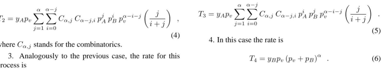
In Figs. 1(a), 1(b) and 1(c) we show the mean-field re-sults along with the Monte Carlo simulations, for the order parameterpv for the linear, square and cubic lattices. This figure clearly indicates that a close agreement between the results of mean-field and Monte Carlo calculations is ob-served far away of the critical point. As we can see in Figs.
1(b) and 1(c) the critical point obtained in the pair approxi-mation and through Monte Carlo simulations are almost the same. However, the slope of the curves at the critical point are rather different. The simulations will be detailed in the next section. ForyA> yActhe system is in an active steady state, while for valuesyA < yAc the system is trapped into an absorbing state, where the surface is completely poisoned by monomers of the speciesB.
III
Static Monte Carlo simulations
In this section we give a brief description of the method we used. The results of simulations were obtained through the following algorithm: we randomly choose a site from the list of empty sites of the lattice and select, with probability
yA, a monomer Ato be adsorbed. If no one of the near-est neighbor sites of the selected site are occupied byAnor
B monomers, then this empty site becomes occupied by a monomerAand the number of empty sites is decreased by one. Else, if there are some monomers in its neighborhood, then a reaction (A+A) or (A+B) will take place with prob-abilityΠAA(ΠAB ), and the list of empty sites is increased by one. On the other hand, with probabilityyB= 1−yA, a
Bmonomer is deposited on the empty site. Then, we search for Amonomers in its neighborhood. If more than oneA
(a)
0.5 0.6 0.7 0.8 0.9 1
y
A0 0.2 0.4 0.6 0.8
p
v L = 256L = 1024 L = 4096 L = 16384 site mean field pair mean field
(b)
0.5 0.6 0.7 0.8 0.9 1
y
A0 0.2 0.4 0.6 0.8
p
v site mean fieldpair mean field L = 16 L = 32 L = 64 L = 128
(c)
0.5 0.6 0.7 0.8 0.9 1
y
A0 0.2 0.4 0.6 0.8 1
p
v site mean fieldpair mean field L=8 L=16 L=24 L=32
Figure 1. Fraction of empty sites as a function of the parameter
yA. The solid and dotted lines correspond to the mean field
ap-proximations. The symbols represent the results of Monte Carlo simulations for various lattice sizesL. Linear lattice (a), square lattice (b) and cubic lattice (c).
Amonomer is found, thenBremains adsorbed. In order to improve the efficiency of the algorithm we use a continuous time Monte Carlo procedure, where the time per event is no longer constant. If at a given instant of time the number of vacant sites isNv, the selection from this list corresponds to a time incrementN−1
v . All the simulations started with an empty lattice and the time required for a finite system to be-come poisoned depends on the lattice size and on the value ofyA. For the lattice sizes we consider, we expect that, due to the fluctuations, a surface fully covered will be observed for any value ofyAfor sufficiently long times. The absorb-ing state is the only stable state. However, foryA larger than the critical value, the system can be found in a reactive steady state, until a large fluctuation drive it to a poisoned state. This reactive steady state is indeed a metastable state. For these metastable states we compute the order parameter (fraction of vacant sites) which exhibits fluctuations around the mean value. We performed simulations for the various lattice sizes, and we considered detailed calculations near the transition point. The simulations showed that the system exhibits a continuous phase transition between an absorbing state, which is poisoned by monomers of the typeB, and an active steady state.
To obtain the critical exponents of the model we per-formed a finite-size scaling analysis for the order parameter
pv. We assume that it is a generalized homogeneous func-tion of the variablesLand∆ = yA −yAc. We suppose [18, 28] that in the critical region, the order parameter be-haves as
pv ∼L−β/ν⊥Φ
³
∆L1/ν⊥´ , (26)
whereΦis a scaling function with the properties that at the critical pointΦ(0)∼ 1, and thatΦ(x)∼xβ, forx → ∞. The latter property recovers the power law behavior of Eq. (13) which is valid for a system of infinite size near its crit-ical point. The exponentν⊥is the correlation length
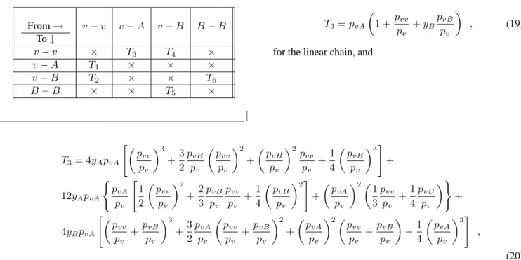
expo-nent and measures the correlations of the order parameter over the surface. At the critical point, a log-log plot ofpv versusLmust be a straight line with slope−β/ν⊥. Figs.
2(a), 2(b) and 2(c) show the log-log plots ofpvversusL, for the linear, square and cubic lattices, respectively. The error bar for each point is not included in these plots. The data points give the valueyAc(d= 1) = 0.63743(7),yAc(d =
2) = 0.5140(5)andyAc(d= 3) = 0.5004(1)for the critical value of the parameteryAfor the three lattices. The values of the critical exponent ratio areβ/ν⊥ = 0.25(1),0.80(2)
and1.40(2), for the linear, square and cubic lattices, respec-tively. These values were calculated by linear fittings to the data points of the simulations including their error bars.
In order to carry out a finite-size scaling analysis for the order parameter, a number of independent runs were done near the transition point for each lattice size, and ford= 1,
(a)
256 1024 4096 16384
L
0.1250.25
p
v yA= 0.6373
yA= 0.6374 yA= 0.63743 yA= 0.6375 yA= 0.6376
(b)
16 32 64 128
L
0.03125 0.0625 0.125 0.25
p
v yA= 0.5130 yA= 0.5135 yA= 0.5140yA= 0.5145
yA= 0.5150
(c)
16 32 64
L
0.008 0.04 0.2
p
v yA = 0.5003
yA = 0.5004 yA = 0.5005 yA = 0.5006
Figure 2. Log-log plots ofpvversusLfor some values of the
pa-rameteryA(indicated in the figures), near the critical point, for (a)
linear chain, (b) square lattice, and (c) cubic lattice. From the slope of the straight lines we foundβ/ν⊥= 0.25,0.80and1.40, for the linear, square and cubic lattices, respectively.
(a)
0.015625 1 64
∆
L
1/ν⊥2 4
p
vL
β/ν
⊥
L= 256 L= 1024 L= 4096 L= 16384
(b)
0.015625 0.125 1 8
∆
L
1/ν⊥2 4 8 16 32
p
vL
β/ν
⊥
L = 16 L = 32 L = 64 L = 128
(c)
0.01 0.1 1
∆
L
1/ν⊥8 16 32 64
p
vL
β/ν
⊥
L = 16 L = 32 L = 64
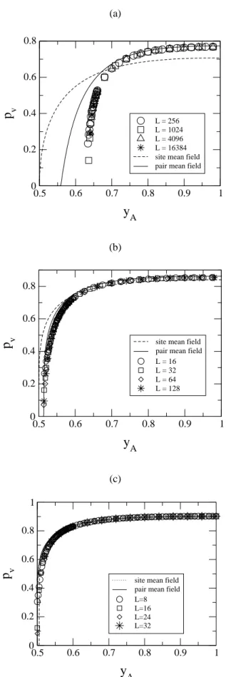
Figure 3. Collapse of the data points for the order parameterpv
for different lattice sizesLfor the linear chain (a), square (b) and cubic (c) lattices. The figure is a log-log plot ofpvLβ/ν⊥ versus ∆L1/ν⊥. The slope of the solid lines, which is the asymptotic be-havior ofpvLβ/ν⊥, givesβ= 0.27,0.57and0.80for the linear,
of 100surviving samples. We have plotted, in Fig. 3, the quantity pvLβ/ν⊥ versus ∆L1/ν⊥ in a log-log scale, for various lattice sizes and dimensions. Figs. 3(a), 3(b) and 3(c) correspond to the simulations performed for the linear, square and cubic lattices, respectively. As we can see, the data for the different lattice sizes, in each plot, collapse very well, suggesting the correctness of the scaling form of Eq. (26). Thus, for large values of the argument of the function
Φin Eq. (26), the data should fall on a straight line with slopeβ.
The collapse of the data points was obtained with the following values of the parameters: β = 0.27(2), ν⊥ =
1.07(3) and yAc = 0.6375(1) for the linear chain, β =
0.58(3), ν⊥ = 0.72(5) and yAc = 0.5141(2) for the square lattice, andβ = 0.80(1),ν⊥ = 0.58(1)andyAc =
0.5004(1)for the cubic lattice. We observe that the ratios
β/ν⊥are the same as those found in Fig. 2. The best values
of the static critical exponents of the Directed Percolation [36] are listed in the table IV.
Table IV. Best values for the static critical exponents of the directed percolation universality class.
critical
exponent d= 1 d= 2 d= 3
β 0.276486(8) 0.584(4) 0.81(1)
ν⊥ 1.096854(4) 0.734(4) 0.581(5)
As we can see, there is a good agreement between the values we found in our static Monte Carlo simulations and those of the DP. This is a good evidence that our catalytic reaction model with competing reactions is in the same uni-versality class of the Directed Percolation.
IV
Dynamic Monte Carlo
simula-tions
We also studied the dynamical critical behavior of the model by introducing a suitable time variable. It is defined as being the mean time required for the system to become completely poisoned. Firstly, we define the time for a selected sample to become poisoned, that is,
τs=
P
ttpv
P
tpv
. (27)
This particular function depends on the linear sizeLof the system and on the parameteryA. Then, we take an average over all the independent samples, getting the quantity
τ =< τs >s, which is assumed to have the scaling form [18, 28]
τ∼Lzφ³∆L1/ν⊥´ . (28)
Albano and Marro [37] have proposed a phenomenolog-ical scaling approach for the poisoning time at the first order transition of the monomer-dimer reaction model. In their approach this time diverges logarithmically with the linear lattice size and algebraically with the distance to the coex-istence point. In Eq. (28) the scaling functionφis assumed to behave asφ(0)∼1at the critical point, so that a log-log
plot ofτversus the system sizeLis a straight line with the slopez. This result is displayed in our Fig. 4 for the lin-ear chain (a), square (b) and cubic (c) lattices. From these figures we obtain z = 1.54(5) andyAc = 0.6375(1)for the linear chain,z = 1.68(6)andyAc = 0.5142(2)for the square lattice, andz = 1.94(2)andyAc = 0.5006(1)for the cubic lattice. Eq. (28) must be consistent with the def-inition of theν||exponent: in the limit of a system with an
infinite lattice size (L→ ∞) the characteristic time diverges asτ ∼(yA−yAc)
−ν||. So, thezand theν
||exponents are
related byz=ν||/ν⊥.
Another way to get information about the critical expo-nents at the critical point, is to consider, for a fixed timet, all the samples (the surviving ones and those which entered the absorbing state). Definingδas the average of the order pa-rameter over many samples, this quantity will depend only on the system sizeLand on time. For the long time behav-ior and for a large system size one can assume the following scaling form
δ∼L−β/ν⊥ψ(t/Lz) . (29)
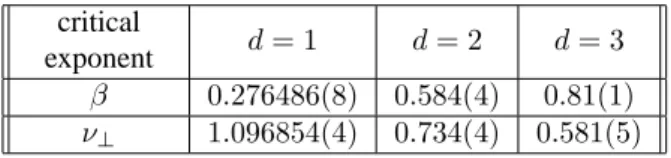
We have plotted, in Fig. 5, δLβ/ν⊥ versus t/Lz on
a log-log scale. The data points collapse very well for
β/ν⊥ = 0.25(1), z = 1.55(2) andyAc = 0.6375(1)in the linear chain case. The values used for the square lattice wereβ/ν⊥ = 0.80(1),z= 1.66(7)andyAc = 0.5141(1). In the cubic lattice the collapse was obtained by choosing
β/ν⊥ = 1.40(1),z = 1.95(1)andyAc = 0.5005(2). All these values are consistent with the previous ones we have found by employing the other manner of collapsing the or-der parameter data. As we can see from these figures, for
t < Lz the data points collapse onto a straight line with the slope−β/ν|| =−0.15(1),−0.48(2)and−0.71(4)for
the linear chain, square and cubic lattices, respectively. Fi-nally, from these ratios, we can estimate the value of the critical exponentν||. We found the values1.8(1)for the
lin-ear chain,1.21(8)for the square lattice and1.13(8)for the cubic lattice. In Fig. 5(c), the data fall on a straight line only in a small region. This fact is due to small lattice sizes used ind= 3.
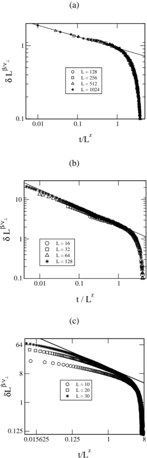
Another way of studying the dynamical critical behav-ior of the model is by employing an epidemic analysis [29, 30, 31]. We measured the survival probabilityP(t), the number of empty sitesnv(t), and the mean square displace-ment from the originR2(t), from an initial state containing only a single empty site at the center of the lattice. Then, we followed the time evolution of many samples with this initial condition until a maximum timetmax= 10000time steps in the linear chain case,tmax = 2500time steps for the square lattice, andtmax = 5000time steps for the cu-bic lattice. For the linear chain and square lattice, one time step was defined by100changes in the configuration of the system, which could be an adsorption or a chemical reaction event. For the cubic lattice, one time step was defined by10
(a)
256 1024 4096
L
10000 1e+05 1e+06
τ
yA= 0.6373
yA= 0.6374 y
A= 0.6375
yA= 0.6376
yA=0.6377
(b)
16 32 64 128
L
256 1024 4096 16384
τ
yA= 0.5136 y
A= 0.5138
y
A= 0.5140
yA= 0.5142
yA= 0.5144
yA= 0.5146
(c)
8 16
L
64 256 1024
τ
yA = 0.5003
yA = 0.5004 yA = 0.5005 yA = 0.5006
yA = 0.5007 yA = 0.5008 yA = 0.5009 yA = 0.5010
Figure 4. Log-log plots ofτ versusLfor some values of the pa-rameteryA (indicated in the figures), near the critical point. In
figure (a), for the linear chain, the slope of the straight line gives
z= 1.54, while for the square (b) and cubic (c) lattices,zis1.68
and1.94, respectively.
(a)
0.01 0.1 1
t/Lz
0.1 1
δ
L
β/ν
⊥
L = 128 L = 256 L = 512 L = 1024
(b)
0.01 0.1 1
t / Lz
0.1 1 10
δ
L
β/ν
⊥
L = 16 L = 32 L = 64 L = 128
(c)
0.015625 0.125 1 8
t/Lz
0.125 1 8 64
δ
L
β/ν
⊥
L = 10 L = 20 L = 30
Figure 5. Collapse of the data points for the dynamical behavior of the order parameter at the critical point. For the linear chain (a), a good collapse was obtained withβ/ν⊥= 0.25,z = 1.55, and
yAc = 0.6375. The slope of the straight line isβ/ν||= 0.15. A good collapse is obtained for the square lattice (b), with the values
β/ν⊥ = 0.80,z = 1.66andyAc = 0.5141. The slope of the
straight line givesβ/ν||= 0.48. In the case of cubic (c) lattice we foundβ/ν⊥= 1.40,z = 1.95andyAc = 0.5005. The slope of
From the scaling ansatz for the DP class and similar models [38, 39], the physical quantities of interest depend on the relevant parameters →r,tand∆ = yA−yAc, only through the scaling variablesr2t−ζ and∆t1/ν||, times some
power ofr2,tor∆. In the scaling regime, the local fraction of empty sites, averaged over all trials, surviving or not, can be written as
pv
³→
r , t´∼tη−ζd/2F³r2t−ζ,∆t1/ν|| ´
, (30) and the survival probability is expected to behave as
P(t)∼t−δΦ³∆t1/ν||´ , (31)
whereν||is the critical exponent associated with the
diver-gence of the temporal correlation length. From equation Eq. (30) we can calculate the number of empty sites,nv(t), and the mean square spreading of the origin,R2(t),
nv(t) =
Z
pv
³→
r , t´ddr , (32)
R2(t) = 1
nv(t)
Z
r2pv
³→
r , t´ddr . (33)
These equations can be cast in the following form
nv(t) ∼ tηΨ
³ ∆t1/ν||
´
, (34)
R2(t) ∼ tζΘ³∆t1/ν||´ . (35)
Here,δ,ηandζare the dynamical critical exponents of the model. The exponent ζ is related to the critical exponent
z, that governs the divergence of the characteristic time, by
ζ = 2/z. Here,Φ,ΨandΘare scaling functions with the property that, at the critical point, they assume a constant value, that is, they are nonsingular functions at the critical point. At the critical point, Eqs. (31), (34) and (35) assume asymptotic power laws
P(t) ∼ t−δ , (36)
nv(t) ∼ tη , (37)
R2(t) ∼ tζ . (38) Log-log plots of these quantities, at the critical point, must be straight lines with slopes giving the corresponding critical exponents. These plots are shown in Figs. 6(a), 6(b) and 6(c), for the linear chain, square and cubic lattices, re-spectively. In each plot of Fig. 6(a) we have three curves. Each curve, from top to bottom, is associated with the values
yA= 0.6376,yA= 0.6375andyA = 0.6374. The straight line gives the critical valueyAc(d= 1) = 0.6375(1). From each plot we obtain δ = 0.160(3), η = 0.314(2) and
ζ = 1.260(1). In each plot of Fig. 6(b) the curves were built with the valuesyA= 0.5145,0.5142and0.5139. The critical value isyAc= 0.5142(3)and the dynamical critical exponents in two dimensions areδ= 0.47(1),η = 0.23(1)
andζ = 1.12(1). For the Fig. 6(c) the curves, from top to
bottom correspond to the valuesyA= 0.5005,yA= 0.5004 andyA = 0.5003and the dynamical critical exponents are
δ= 0.71(4),η= 0.09(7)andζ= 1.03(1). (a)
0.125 0.25
P(t)
4 8 16
nv
(t)
100 1000 t 100
1000 10000
R
2 (t)
(b)
0.00781 0.01563
P(t)
2 4 8
nv
(t)
256 1024
t
256 1024
R
2 (t)
(c)
0.001 0.01
P(t)
0.5 1 2
nv
(t)
64 256 1024 t
100 1000
R
2 (t)
Figure 6. Log-log plots for the quantitiesP(t),nv(t)andR2(t)
It is also possible to find the values of the critical ex-ponents by looking at the local slopes. Consider, for in-stance, Eq. (31). By changing the scale of the time vari-able by an integer m we can write, at the critical point,
P(mt) =m−δP(t). From this, we have
−δ(t) = log [P(mt)/P(t)]
logm , (39)
with similar expressions for the exponentsηandζ. At large times, the local slopeδ(t)assumes the following asymptotic behavior
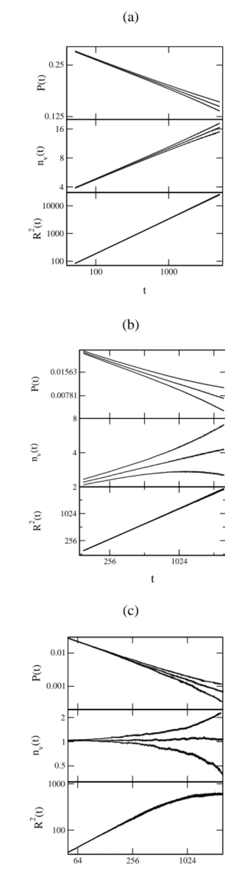
δ(t) =δ+at−θ+bt−φ+· · · , (40) whereθ andφ are corrections to scaling due to the finite size of the lattice. We also estimated the critical exponents by plotting the local slopes versus1/tand extrapolating to
1/t → 0. The plots for the local slopeδ(t)are shown in Fig. 7(a), for the linear chain, in Fig. 7(b), for the square lattice and in Fig. 7(c) for the cubic lattice, where we used
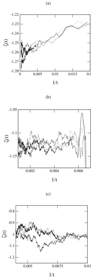
m= 2. The curves in each plot correspond to different val-ues of the parameteryAaround the critical valueyAc, which is the central curve in the plot. From these figures we esti-mate the valuesδ = 0.163(7),0.46(1)and0.71(3)for the linear chain, square and cubic lattices. We also plotted the local slopeη(t)versus1/tfor the three lattices in the Figs. 8(a), 8(b) and 8(c). From these figuresη(d= 1) = 0.31(5),
η(d = 2) = 0.23(1) and η(d = 3) = 0.12(4). Fi-nally, in Fig. 9, we plotted the local slopeζ(t)versus1/t
for the linear chain 9(a), square 9(b) and cubic 9(c) lat-tices. These plots give the values ζ(d = 1) = 1.26(1),
ζ(d= 2) = 1.13(2)andζ(d= 3) = 1.03(1).
Our calculated dynamical critical exponents agree with those found for the Directed Percolation in one, two and three spatial dimensions. The best values of these critical exponents [36] are listed in the table V.
Table V. Best values for the dynamic critical exponents of the directed percolation universality class.
critical
exponent d= 1 d= 2 d= 3
z 1.580745(10) 1.76(3) 1.90(1)
ν|| 1.733847(6) 1.295(6) 1.105(5)
δ 0.159464(6) 0.451 0.73
η 0.313686(8) 0.230 0.12
ζ 1.26523 1.13636 1.05263
(a)
0 0.0025 0.005
1/t
0.12 0.14 0.16 0.18 0.2
δ
(t)
(b)
0.002 0.004 0.006
1/t
0.3 0.35 0.4 0.45 0.5 0.55 0.6 0.65
δ
(t)
(c)
0 0.005 0.01
1/t
0.5 1 1.5
δ
(t)
Figure 7. Local slope δ(t) for the linear chain (a), square (b) and cubic (c) lattices. From these plots we estimate the value of the critical exponentδ, whose values areδ(d = 1) = 0.163(7),
(a)
0 0.0025 0.005
1/t
-0.35 -0.325 -0.3 -0.275 -0.25
η
(t)
(b)
0.002 0.004 0.006
1/t
-0.5 -0.4 -0.3 -0.2 -0.1 0
η
(t)
(c)
0.005 0.01
1/t
-0.5 -0.25 0 0.25 0.5
η
(t)
Figure 8. Local slope η(t) for the linear chain (a), square (b) and cubic (c) lattices. From these plots we estimate the value of the critical exponent η, whose values areη(d = 1) = 0.31(5),
η(d= 2) = 0.23(1)andη(d= 3) = 0.23(12).
(a)
0 0.005 0.01 0.015 0.02
1/t
-1.28 -1.27 -1.26 -1.25 -1.24 -1.23 -1.22
ζ
(t)
(b)
0.002 0.004 0.006
1/t
-1.15 -1.1 -1.05
ζ
(t)
(c)
0.005 0.0075 0.01
1/t
-1.2 -1.1 -1 -0.9 -0.8
ζ
(t)
Figure 9. Local slopeζ(t) for the linear chain (a), square (b) and cubic (c) lattices. From these plots we estimate the value of the critical exponentζ, whose values areζ(d = 1) = 1.26(1),
V
Conclusions
We have studied a competitive reaction model between monomers on a catalytic surface. The model can be viewed as being a mixture of the autocatalytic and the monomer-monomer reaction models. We have considered the site and the pair mean-field approximations to obtain the steady states and a qualitative picture of the critical behavior of the model in one, two and three spatial dimensions. The model displays a continuous phase transition into a single absorb-ing state. The critical point obtained via pair approximation agree very well with that found by Monte Carlo simulations in two and three dimensions. By employing finite-size scal-ing arguments, we determined the static and dynamic critical exponents of the model. All the values we have found are in agreement with those of the Directed Percolation (DP) in
(d+ 1) dimensions. This was indeed expected, since the phase transition from the active to the single absorbing state is one in which the concentration of vacancies goes con-tinuously to zero. Although our model can not be mapped onto the DP, they are equivalent concerning the static and dynamic critical behavior. This is a strong evidence in favor of the universality: models with different dynamical rules exhibit the same critical behavior. The essential characteris-tic shared by these models is a continuous phase transition into an absorbing state. The DP conjecture asserts that mod-els with a continuous phase transition into an absorbing state belong generically to the DP universality class. In summary, based on the values we have found for the static and dy-namic critical exponents, and on the DP conjecture, we can conclude that our model belongs to the same universality class of the DP.
Acknowledgments
This work was supported by the Brazilian agency CNPq.
References
[1] R. N. Mantegna and H. E. Stanley, An Introduction to
Econo-physics: Correlation and Complexity in Finance, (Cambridge
University Press, Cambridge, 2000).
[2] J. V. Andersen and D. Sornette, Eur. Phys. J. B 31, 141 (2003).
[3] R. Dickman, Phys. Rev. Lett. 90, 108701 (2003).
[4] R. Dickman, T. Tom´e and M. J. de Oliveira, Phys. Rev. E 66, 016111 (2002).
[5] T. Tom´e and M. J. de Oliveira, Phys. Rev. Lett. 86, 5643 (2001).
[6] J. Krug, Adv. Physics 46, 139 (1997).
[7] A. -L. Barabasi and H. E. Stanley, Fractal concepts in surface
growth, (Cambridge University Press, Cambridge, 1995).
[8] D. Chowdhury, L. Santen, and A. Schadschneider, Phys. Rep.
329, 199 (2000).
[9] V. S. Leite, and W. Figueiredo, Phys Rev. E 66, 46102 (2002).
[10] W. Figueiredo and B. C. S. Grandi, Braz. J. of Phys. 30, 58 (2000).
[11] M. Godoy, and W. Figueiredo, Phys. Rev. E 66, 036131 (2002).
[12] Kenneth G. Wilson, Phys. Rev. B 9, 3174 (1971); Phys. Rev. B 9, 3184 (1971).
[13] J. Marro and R. Dickman, Nonequilibrium phase transitions
in lattice models, (Cambridge University Press, Cambridge,
1999).
[14] Nonequilibrium statistical mechanics in one dimension, edited by V. Privman, (Cambridge Universty Press, Cam-bridge, 1997).
[15] F. Schl¨ogl, Z. Physik 253, 147 (1972).
[16] R. M. Ziff, E. Gulari, and Y. Barshad, Phys. Rev. Lett. 56, 2553 (1986).
[17] R. M. Ziff, and B. J. Brosilow, Phys. Rev. A 46, 4630 (1992); I. Jensen, H. C. Fogedby, and R. Dickman, Phys. Rev. A 41, 3411 (1990); R. Dickman and M. Burschka, Phys. Lett. A
127, 132 (1988); E. V. Albano, Surf. Sci. 306, 240 (1994); J.
W. Ewans, and M. S. Miesch, Phys. Rev. Lett. 66, 833 (1991); V. S. Leite, B. C. S. Grandi, and W. Figueiredo, J. Phys. A: Math. Gen. 34, 1967 (2001).
[18] E. C. da Costa, and W. Figueiredo, J. Chem. Phys. 117, 331 (2002).
[19] E. C. da Costa, and W. Figueiredo, J. Chem. Phys. 118, (2003).
[20] R. M. Ziff and K. Fichthorn, Phys. Rev. B 34, 2038 (1986).
[21] P. Meakin and D. J. Scalapino, J. Chem. Phys. 87, 731 (1987).
[22] P. L. Krapivsky, J. Phys. A: Math. Gen. 25, 5831 (1992).
[23] H. Park, J. K¨ohler, In-Mook Kim, D. ben-Avraham and S. Redner, J. Phys. A: Math. Gen. 26, 2071 (1993).
[24] D. ben-Avraham, D. Considine, P. Meakin, S. Redner, and H Takayasu, J. Phys. A: Math. Gen. 23, 4297 (1990).
[25] K. S. Brown, K. E. Bassler, and D. A. Browne, Phys. Rev. E
56, 3953 (1997).
[26] J. Cort´es, H. Puschmann, and E. Valencia, J. Chem. Phys 106, 1467 (1997).
[27] D. A. Browne and P. Kleban, Phys. Rev. A 40, 1615 (1989).
[28] T. Aukrust, D. A. Browne, and I. Webman, Phys. Rev. A 41, 5294 (1990).
[29] P. Grassberger, J. Phys. A 22, 3673 (1989).
[30] I. Jensen, J. Phys. A, 26, 3921 (1993).
[31] I. Jensen, Phys. Rev. E 50, 3623 (1994).
[32] H. Hinrichsen, Braz. J. of Phys. 30, 69 (2000).
[33] E. C. da Costa and W. Figueiredo, Phys. Rev. E 61, 1134 (2000).
[34] A. G. Dickman, B. C. S. Grandi, W. Figueiredo, and R. Dick-man, Phys. Rev. E 59, 6361 (1999).
[35] G. L. Hoenicke, and W. Figueiredo, Phys. Rev. E 62, 6216 (2000).
[36] H. Hinrichsen, Adv. Phys. 49, 815 (2000).
[37] E. V. Albano and J. Marro, J. Chem. Phys. 22, 10279 (2000).
[38] P. Grassberger, Z. Physik B 47, 465 (1982).