Variable Survival Exponents in History-Dependent
Random Walks: Hard Movable Reflector
Ronald Dickman
1, Francisco Fontenele Araujo Jr.
1, and Daniel ben-Avraham
2 1Departamento de F´ısica, ICEx, Universidade Federal de Minas Gerais,C.P. 702, 30.161-970, Belo Horizonte - Minas Gerais, Brazil 2Physics Department, Clarkson University, Potsdam, NY 13699-5820, USA
Received on 1st April, 2003
We review recent studies demonstrating a nonuniversal (continuously variable) survival exponent for history-dependent random walks, and analyze a new example, the hard movable partial reflector. These processes serve as simplified models of infection in a medium with a history-dependent susceptibility, and for spreading in systems with an infinite number of absorbing configurations. The memory may take the form of a history-dependent step length, or be the result of a partial reflector whose position marks the maximum distance the walker has ventured from the origin. In each case, a process with memory is rendered Markovian by a suitable expansion of the state space. Asymptotic analysis of the probability generating function shows that, for larget, the survival probability decays asS(t)∼t−δ, whereδvaries with the parameters of the model. We report new
results for ahardpartial reflector, i.e., one that moves forward only when the walker does. When the walker tries to jump to the site R occupied by the reflector, it is reflected back with probabilityr, and stays at R with probability1−r; only in the latter case does the reflector move (R→R+1). For this model,δ= 1/2(1−r), and
becomes arbitrarily large asrapproaches 1. This prediction is confirmed via iteration of the transition matrix, which also reveals slowly-decaying corrections to scaling.
I
Introduction
Random walks with absorbing or reflecting boundaries, or with memory, serve as important models in statistical physics, often admitting an exact analysis. Among the many examples are equilibrium models for polymer adsorption [1-4] and absorbing-state phase transitions [5]. Another mo-tivation for the study of such problems is provided by the spreading of an epidemic in a medium with a long memory [6, 7].
In addition to the intrinsic interest of such an infection with memory, our study is motivated by the spread of ac-tivity in models exhibiting an infinite number of absorbing configurations (INAC), typified by the pair contact process [8, 9]. Anomalies in critical spreading for INAC, such as continuously variable critical exponents, have been traced to a long memory in the dynamics of the order parameter,
ρ, due to coupling to an auxiliary field that remains frozen in regions whereρ = 0[9, 10]. INAC appears to be par-ticularly relevant to the transition to spatiotemporal chaos, as shown in a recent study of a coupled-map lattice with “laminar” and “turbulent” states, which revealed continu-ously variable spreading exponents [11].
Grassberger, Chat´e and Rousseau [6] proposed that spreading in INAC could be understood by studying a model
with a unique absorbing configuration, but in which the spreading rate of activity into previously inactive regions is different than for revisiting a region that has already been ac-tive. In light of the anomalies found in spreading in models with INAC or with a memory, we are interested in study-ing the effect of such a memory on the scalstudy-ing behavior in a model whose asymptotic behavior can be determined ex-actly. Of particular interest is the survival probabilityS(t) (i.e., not to have fallen into the absorbing state up to timet). In the present work, we review previous results on sur-vival of random walks with memory, and analyze the asymp-totic behavior of a random walk subject to a hard movable reflector. On the basis of an exact solution for the probability generating function, we obtain the decay exponentδ.
The balance of this paper is organized as follows. Sec-tion II reviews previous results on variable survival expo-nents for random walks with memory. In Sec. III we define the hard reflector model and obtain a formal solution for the generating function. An asymptotic analysis of this func-tion is presented in Sec. IV, leading to an expression for the decay exponentδin terms of the reflection probability
II
Variable survival exponents in
ran-dom walks with memory
Relatively simple random walk problems often serve as re-duced examples of much more complicated many-body phe-momena. So it is with phase transitions between an active and an absorbing state. In these systems [5, 12] the station-ary state of a Markov process exhibits (in the infinite-size limit) a phase transition from a frozen, inactive regime to one with sustained activity, as a control parameter is var-ied. Broadly speaking, the control parameter represents the reproduction rate of activity (A→2A) relative to its extinc-tion (A→0). The simplest examples are the contact process [13] and directed percolation (DP).
Consider now, instead of the stationary state, thespread of activity from a localized source, in an infinite system. In the subcritical regime (for which the only stationary state is the inactive, absorbing one), the initial activity decays (typ-ically, exponentially fast), while in the supercritical regime there is a finite probability for it to spread indefinitely. Just at the critical point, one finds a scale-invariant evolution: the survival probability S(t), the integrated activityn(t), and the mean-square distance, R2(t), of the activity from the initial seed, all follow asymptotic power laws.
The question of survival arises naturally in the context of a random walk in the presence of an absorbing boundary. The survival probabilityS(t)is the probability never to have visited an absorbing boundary until time t. The simplest example is a one-dimensional random walkxt (in discrete time) on the non-negative integers, with the origin absorb-ing, andx0 ≥ 1. Let the walker jump, at each time step, to the right (xt+1=xt+ 1) with probabilityp, and the left (xt+1 = xt−1) with probability q = 1−p. Ifp < q then the survival probability decays exponentially, while for
p > qit approaches (again exponentially) a nonzero value, so that the walker has a finite probability to escape to infin-ity. In the absence of drift (p = q = 1/2),S(t) ∼ t−1/2 for larget; associated with this power-law decay is an infi-nite mean lifetime. In the analogy with an absorbing-state phase transition, p = 1/2 evidently marks the transition, with extinction certain forp≤1/2, and a finite asymptotic survival probability forp >1/2. The same qualitative situ-ation holds in the contact process, starting for example from a single active site [5].
The analogy is in factexactfor the rather special case ofcompact directed percolation(CDP), in which active re-gions are delimited by independent random walks that anni-hilate on contact. (CDP is a particular limit of the Domany-Kinzel model [14].) In this case ‘drift’ corresponds to a tendency of the walkers at the boundaries of an active re-gion to approach, or separate from, one another; the critical point corresponds to zero drift, or unbiased random walk-ers (p= 1/2). Initializing CDP with a finite interval (say, 1, 2,...,m) of active sites, is equivalent to placing random walkers (xt andyt) at 0 and m+ 1. The active region at any subsequent time corresponds to the interval between the walkersxtandyt; the process ends when the two meet. To
make the analogy between CDP and a random walk with the origin absorbing complete, we may fixxt= 0for all times, so that only the right frontier of the active region is free to fluctuate, while the left frontier is pinned, as it were, at a wall.
Given the connection with phase transitions, we shall think of the power law for the survival probabilty as defin-ing a critical exponent, and writeS(t) ∼ t−δ. The main interest of the examples discussed in this paper is that the exponentδcan be shown tovary continuouslyas a function of a parameter. This in turn may help to understand scaling in more complex examples, such as the pair contact process [8], for which a variable survival exponent has been reported numerically, but cannot be established rigorously.
Random walk models exhibiting variable survival expo-nents fall in two classes. In one, the position of the absorb-ing boundary is a given (deterministic) function of time. A random walk in the presence of such a boundary defines a nonstationary stochastic process. The second class (which is our principal interest here) involvesmemory, either in the form of a reflector that moves when it encounters the walker, or of a history-dependent step length.
We begin with a brief review of the first class. In a highly readable paper, Krapivsky and Redner [15] consid-ered what happens when a random walker on the line is sub-ject to two absorbing boundaries,R(t)andL(t), which are prescribed functions of time (initially the walker is at the origin). The absorbers are initially near the origin, and fol-lowR(t) =a+ (At)α,L(t) = −R(t). Forα > 1/2, the absorbers rapidly leave the region explored by the walker, which therefore enjoys a finite probability of survival as
t→ ∞. If the absorbers are stationary we of course expect
S(t)to decay exponentially; but if their motion is charac-terized by0 < α < 1/2, this changes to astretched expo-nentialdecay,S ∼ exp[−t1−2α]. Forα= 1/2, the ‘safe’ region expands with the same power law as the region ex-plored by the walker. The result is power-law decay of the survival probability, with a variable exponent which depends onA.
The problem studied by Krapivsky and Redner may be pictured as a random walk confined to a parabola in thet−x
plane, whose equation (fort ≥ 0) isx= ±(At)α. When
α= 1/2, as noted, there is power-law decay ofS(t), with a nonuniversal exponent. Similar conclusions apply for DP and for directed self-avoiding walks [16], and for CDP [17], when these processes are confined to a fixed parabola.
We now turn to studies of a random walk subject to some special condition when it enters virgin territory, i.e., when it attempts to visit a site for the first time. Here there is no fixed confining boundary; the condition depends on the his-tory of the walk. But since the region explored by the walker grows∝t1/2, it effectively creates its own parabola.
occupied by the reflector, it is reflected one step to the left with probabilityr(it remains at its new location with proba-bility1−r); in either case, the reflector is pushed forward one site in this encounter. The survival exponentδ= (1+r)/2in this process [18]. Since the reflector effectively records the spanof the walk (i.e., the rightmost site yet visited), its inter-action with the walker represents a memory. We shall refer to this model as thesoft reflector, to highlight the fact that the refector obligingly moves forward, even if the walker is reflected back. Note that in this caseδnever exceeds unity.
The analysis of the random walk with soft reflector was subsequently extended to compact directed percolation [19]. The active region initially consists of a single site (the ori-gin), and, as already noted, is bounded by a pair of inde-pendent, unbiased random walkers, originally atx= 0and
x = 1. The two walkers are subject to movable partial (“soft”) reflectors, such that the walker on the right is re-flected toward the left and vice-versa. The results for the survival exponent are qualitatively similar to those for the single walker, but δnow varies between 1/2 and 1.160 as the reflection probability r varies between zero and one. The results (coming in this case from iteration of the transi-tion matrix, rather than from an asymptotic analysis of the generating function), are well fit by the simple expression
δ = 1/2 + 2r/3; small but significant deviations from this simple formula are found, however. CDP with reflectors has so far defied exact analysis, and the reason for the specific valueδ= 1.160forr= 1is not understood.
Most recently, the methods developed in Ref. [18] were applied to a one-dimensional random walk with memory of a different form: if the target site xlies in the region that has been visited before (that is, ifxitself has been visited, or lies between two sites that have been visited), then the step length isv; otherwise the step length isn. In this case one findsδ=v/2n[20]. Thusδcan take any rational value between zero and infinity.
With this background we may now describe the prob-lem to be analyzed here as a random walk subject to ahard partial, movable reflector. This is because the reflector now moves forward if and only if the walker succeeds in occu-pying the new position; when the walker is reflected, the reflector maintains its position. This, as will be shown, can lead to much larger values ofδthan in the soft reflector case. Before embarking on the technical discussion, we sum-marize our approach, as developed in Refs. [18] and [20]. After formulating the problem, we enlarge the state space so that the process becomes Markovian in the expanded rep-resentation [21]. We then write down the equation of mo-tion for the probability distribumo-tion and its associated bound-ary and initial conditions. Since these are discrete models, the equation of motion corresponds to a set of difference equations, first-order in time, and second-order in space. It is convenient to eliminate the time variable by passing to a generating functionPˆ(z)(effectively, a discrete Laplace transform). Using separation of variables, we obtain a for-mal solution for the generating function. Finally, the asymp-totic long-time behavior is found by studying the generating
function for the survival probability in the limitz→1.
III
Model
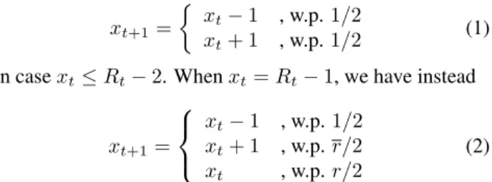
Consider an unbiased, discrete-time random walk on the nonnegative integers, with the origin absorbing. We denote the position of the walker at time t byxt, withx0 = 1. The movement of the walker is affected by the presence of a movable partial reflector, whose position is denoted byRt, withR0= 2. At each time step the walker hops from its cur-rent positionxtto eitherxt+ 1orxt−1with probabilities of 1/2. If, however,xt+1 =Rt, the walker is reflected back toxtwith probabilityr, and remains atxt+1with probabil-ityr ≡1−r; in the latter case the reflector simultaneously moves toRt+ 1. Summarizing, the transition probabilities for the walker are
xt+1= ½
xt−1 , w.p.1/2
xt+ 1 , w.p.1/2 (1) in casext≤Rt−2. Whenxt=Rt−1, we have instead
xt+1 =
xt−1 , w.p.1/2
xt+ 1 , w.p.r/2
xt , w.p.r/2
(2)
The position of the reflector at any moment is given by
Rt= 1 + maxt′≤t{xt′}.
Although the process xt is non-Markovian (since the transition probability into a given site depends on whether it has been visited previously), we can define a Markov pro-cess by expanding the state space to include the variable
yt ≡ Rt−1 = maxt′≤t{xt′}. The state spaceE ⊂ Z2
is given by by
E={(x, y)∈Z2:x≥0, y≥1, x≤y},
as represented in Fig. 1.
✁ ✂ ✄ ☎✝✆✟✞✡✠☞☛☞✌✟✍☞✎ ✆ ✞ ✠ ☛ ✌ ✍ ✎ ✏ ✏ ✏ ✏ ✏ ✏ ✏ ✏ ✏ ✏ ✏ ✏ ✏ ✏ ✏ ✏ ✏ ✏ ✏ ✏ ✏ ✏ ✏ ✏ ✏ ✏ ✏ ✏ ✏ ✏ ✏ ✏ ✏ ✏☞✏ ✑ ✑✓✒ ✑ ✑✓✒ ✑ ✑✓✒ ✑ ✑✓✒ ✑ ✑✓✒ ✑ ✑✓✒ ✔ ✔ ✔ ✔ ✔ ✔ ✔ ✔ ✔ ✔ ✔ ✔ ✔ ✔ ✔ ✔ ✔ ✔ ✔ ✔ ✔ ✔ ✔ ✔ ✔ ✔ ✔ ✔ ✔ ✔ ✔ ✔ ✔ ✔ ✔ ✕✖ ✗✕✖ ✘ ✖
Figure 1. Random walk subject to hard reflector: transitions in the
x-yplane.
P(x, y, t+ 1) = 1
2P(x+ 1, y, t) + 1
2P(x−1, y, t), forx < y−1, (3) withP(x, y,0) =δx,1δy,1. Eq. (3) is subject to two boundary conditions. The first is the absorbing condition forx≤0
P(x, y, t) = 0, forx≤0. (4) The second applies along the diagonalx=y. DefiningD(y, t)≡P(y, y, t), we have
D(y, t+ 1) = 1
2P(y−1, y, t) +
r
2 D(y−1, t) +
r
2D(y, t), fory≥2. (5) Fory= 1the equation is simplyD(1, t+ 1) = (r/2)D(1, t), and sinceD(1,0) = 1, one hasD(1, t) = (r/2)t. Finally, for
x=y−1,
P(y−1, y, t+ 1) = 1
2P(y−2, y, t) + 1
2D(y, t), forx < y−1, (6) We next introduce the generating function:
ˆ
P(x, y, z) =
∞
X
t=0
P(x, y, t)zt. (7)
Multiplying Eqs. (3), (6) byzt, summing overtand shifting the sum index where necessary, one finds that the generating function satisfies
1
zPˆ(x, y) =
1
2Pˆ(x+ 1, y) + 1
2Pˆ(x−1, y), forx≤y−2 (8) 1
zPˆ(y−1, y) =
1 2Dˆ(y) +
1
2Pˆ(y−2, y), forx=y−1, (9) (we drop the argumentz for brevity), whereDˆ(y)is defined by an expression analogous to Eq. (7). The initial condition impliesDˆ(1) = (1−zr/2)−1; the boundary conditions are
ˆ
P(0, y) = 0, (10) and
1
zDˆ(y) =
1
2Pˆ(y−1, y) +
r
2Dˆ(y−1) +
r
2Dˆ(y), fory≥2. (11) Eq. (8) relatesPˆat different values ofx, for the samey. Specifically, on the interior of each line of constanty,Pˆsatisfies a diffusion equation, with a source atx=yand a sink atx= 0. It is therefore natural to attempt separation of variables,
ˆ
P(x, y) = ˆA(x) ˆB(y). (12) Inserting this expression in Eq. (8) one obtains
1
zAˆ(x)−
1
2Aˆ(x−1)− 1
2Aˆ(x+ 1) = 0, (13) withA(0) = 0. The solution satisfying this boundary condition is
ˆ
A(x) =λx−λ−x,
(14) with
λ= 1
z+
r 1
z2−1. (15)
Our next task is to determineBˆ(y); for this we require a relation between generating functions with different arguments
y. Relations of this kind arise along the diagonal, but involve the functionDˆ(y), which we proceed to eliminate. Combining Eqs. (9) and (11), we find
Q(z) ˆD(y) = zr
2 Dˆ(y−1) +
z2
4 Pˆ(y−2, y) (16) where
Q(z) = 1−zr 2 −
z2
Equation (11) may also be written as ³
1−zr2 ´Dˆ(y)−zr2 Dˆ(y−1) = z
2Pˆ(y−1, y), (18) We now multiply Eq. (16) fory−1byβ≡zr/(2−zr)and subtract the result from the same equation fory. This yields
QhDˆ(y)−βDˆ(y−1)i= zr 2
h ˆ
D(y−1)−βDˆ(y−2)i+z 2
4 h
ˆ
P(y−2, y)−βPˆ(y−3, y−1)i . (19) From Eq. (18) we have
ˆ
D(y)−βDˆ(y−1) = z
2−zrPˆ(y−1, y), (20)
allowing us to eliminateDˆ from Eq. (19): 4Q
z(2−zr)Pˆ(y−1, y)−Pˆ(y−2, y) =β ·
2
zPˆ(y−2, y−1)−Pˆ(y−3, y−1)
¸
. (21)
Inserting Eq. (12) one readily finds a recursion relation forBˆ: ˆ
B(y) ˆ
B(y−1) =
zr[2 ˆA(y−2)−zAˆ(y−3)]
(4−2zr−z2) ˆA(y−1)−z(2−zr) ˆA(y−2) . (22) GivenBˆ(1) = ˆD(1)/Aˆ(1)withDˆ(1)andAˆ(y)as found above, Eqs. (12), (14), and (22) represent a complete formal solution for the generating functionPˆ(x, y).
⌈
IV
Asymptotic analysis
Our goal is to find the survival probabilityS(t)for larget. This can be found analysing the associated generating func-tion,
ˆ
S(z) =
∞
X
t=0
S(t)zt (23) in the limitz → 1. Specifically, ifS(t) ∼ t−δ, then the radius of convergence ofSˆ(z)is|z| = 1, and the singular behavior of the generating function asz→1determinesδ. Indeed, in this case, withz= 1−ǫ, we have
ˆ
S ≃
∞
X
t=1
t−δ(1 −ǫ)t
≃ Z ∞
1
dt t−δexp[
−t|ln(1−ǫ)|]
≃ ǫδ−1Γ(1
−δ), (24)
so that the scaling exponent δ can be read off from the power-law dependence ofSˆonǫ = 1−z asǫ→ 0. This simplifies considerably the determination of the long-time asymptotic behavior ofS(t).
The generating functionSˆ has two contributions, com-ing from the “interior” (x < y) and the diagonal:
ˆ
S =
∞
X
y=1 y−1 X
x=1 ˆ
P(x, y) +
∞
X
y=1 ˆ
D(y)
≡ SˆP+ ˆSD. (25)
Using Eq. (20) one readily shows that
ˆ
SD=
z
2−z
∞
X
y=1 ˆ
P(y−1, y)<SˆP , (26)
so that it suffices to analyze the behavior ofSˆP. Consider
ˆ
SP =
∞
X
y=1 ˆ
B(y) y−1 X
x=1 ˆ
A(x). (27)
The sum overxcan be evaluated as y−1
X
x=1 ˆ
A(x) = λ y−1
λ−1 −
λ−y−1
λ−1−1
≃ Λ4 sinh2Λy
2 (28) where in the last step we usedΛ≡lnλ≃√2ǫasǫ→0.
To evaluateSˆPwe also require an expression forBˆ(y)in the limitǫ→0; this can be obtained from Eq. (22). We be-gin by setting all explicit factors ofzequal to unity, since the O(ǫ)corrections thereby discarded do not contribute to the singular behavior ofSˆP. The singular contributions in fact originate from the functionsAˆ, through their dependence on
⌋ ˆ
B(y) ˆ
B(y−1) ≃
r[2 sinh Λ(y−2)−sinh Λ(y−3)]
(3−2r) sinh Λ(y−1)−(2−r) sinh Λ(y−2) . (29)
⌈
Using the identity sinh(a + b) = sinhacoshb + sinhbcosha, and neglecting termsO(Λ2), we obtain
ˆ
B(y) ˆ
B(y−1) ≃
tanh Λy−Λ
tanh Λy+ Λ/r . (30)
Fory ≤ y0 = [2/r] + 1(here[...]denotes the integer part of its argument), we can write, for smallΛ
ˆ
B(y) = ˆB(1) y Y
k=2
k−1
k+ 1/r =CBˆ(1), (31)
whereCdepends onrandy but is independent ofΛ. We shall in fact discard the contribution due toy < y0inSˆP. The reason is that the contribution to the survival probabil-ity from any fixed, finite set of transient states must decay exponentially at long times, and so will not affect our result for the scaling exponent.
Noting thatBˆ(1) = ˆD(1)/Aˆ(1) ∝ 1/Λ, we have, for
y > y0,
ˆ
B(y) =C Λ
y Y
k=y0 ˆ
B(k) ˆ
B(k−1) , (32) whereC is a constant. Since all terms havek ≥ 2/r, we may use Eq. (30) to write, withφk≡tanh Λk,
ln Bˆ(y) ˆ
B(y0) ≃
y X
k=y0
ln 1−Λ/φk 1 + Λ/(rφk)
≃ − µ
1 +1
r
¶ Λ
y X
k=y0 1
φk
. (33)
Approximating the sum by an integral we find
ln Bˆ(y) ˆ
B(y0) ≃
µ 1 + 1
r
lnsinh Λy0
sinh Λy . (34)
Now, inserting Eqs. (28) and (34) in Eq. (27), the gen-erating function forǫ→0is:
ˆ
SP ∼Λ1/r−1
∞
X
y=y0
sinh2Λy/2
sinh1+1/rΛy , (35)
where ‘∼’ denotes asymptotic proportionality asǫ→0. Ap-proximating, as before, the sum by an integral, we have
ˆ
SP ∼Λ1/r−2 Z ∞
Λy0
du sinh
2u/2
sinh1+1/ru. (36)
Since1 + 1/r ≥ 2, the integral converges at its upper limit. Forr < 1/2,1 + 1/r < 3and the integral remains finite asΛ→0. Then
ˆ
SP ∼Λ1/r−2∼ǫ1/(2r)−1, (37) so that the survival probability decays asS(t) ∼ t−δ with
δ = 1/2r. Forr = 1/2, the prefactor in Eq. (36) is inde-pendent ofΛand
ˆ
SP ∼ Z ∞
Λy0
du
u ∼ −ln(1−z). (38)
Expanding the logarithm, we findSˆ(z)∼P
nzn/n, yield-ing directlyS(t)∼t−1. Finally, whenr >1/2,1+1/r >3 and the integral in Eq. (36) contains two principal contribu-tions: one finite (due to the interval from say, 1, to infin-ity), the other arising from the lower limit, and diverging asΛ2−1/r. Combined with the prefactor∝ Λ1/r−2 how-ever, the latter contribution is nonsingular, while the former is again proportional toΛ1/r−2.
Summarizing, the asymptotic survival probability de-cays as a power law,
S(t)∼t−1/2r,
(39) which is the result we set out to prove.
V
Numerical Results
The foregoing analysis provides thet→ ∞scaling behav-ior of the survival probability, but does not indicate the rate of convergence to the asymptotic power law. To determine how the corrections to scaling decay, we iterate the discrete time evolution equation forP(x, y, t)directly. In Fig. 2 we show the decay ofS(t)for reflection probabilityr = 0.85, corresponding toδ = 10/3. For very late times, the graph indeed approaches a power law with the expected exponent. The approach is, however, extremely slow.
Figure 2. Decay of survival probabilityS(t)for reflection proba-bilityr= 0.85(solid curve); the slope of the straight line is -10/3. We have found a particularly simple transformation of variable that appears to take the dominant correction to scal-ing into account. It consists in definscal-ing a shifted time vari-able
T =t+bt1/2, (40) with parameterbadjusted to make the graph ofSversusT
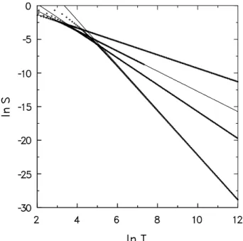
(on log scales) as linear as possible. Fig. 3 shows the sur-vival probability data forr= 1/2, 2/3, 0.75 and 0.85 versus
T (the correspondingbvalues are 1.754, 4.167, 7.042, and 16.67). In each case the numerical data (points) follow the modified power law,
S(T) =AT−δ, (41) to very high precision. [HereAis an amplitude determined by extrapolatingTδS(T)toT → ∞.] The numerical data appear to converge rapidly (faster than a power law) to the fit. While this ‘shifted time’ analysis is for the moment without theoretical basis, it clearly confirms the asymptotic power laws found analytically, and suggests a simple form for describing slowly decaying corrections to scaling.
The slowly decaying correction to scaling would likely frustrate efforts to extract the correct long-time behavior from simulations. Looking at Fig. 2, we see that the asymp-totic power law is barely evident whenS(t)has decayed to
e−15. To obtain even marginally useful simulation data in this situation we would need to perform≥10e15≃3×10⁷ independent realizations of the process, extending to a max-imum time of about 2000 steps. This is feasible for a simple random walk, but becomes a computational challenge for a many-particle system. Thus, if lattice models such as the PCP behave in a manner analogous to what is found for the random walk with a hard reflector, it will be very difficult to confirm power-law scaling in simulations. Data for limited times (or limited samples) may well give the impression of faster than exponential decay ofS(t).
Figure 3. Survival probabilitySas a function of the shifted time variableT, for reflection probabilitiesr= 1/2, 2/3, 3/4 and 0.85 (data points); the straight lines have slopes of 1, 3/2, 2, and -10/3.
VI
Discussion
We have reviewed examples of confined random walks, and random walks with memory, that lead to a continuously vari-able scaling exponent for the survival probability, and anal-ysed in detail the ‘hard reflector’ case. The latter problem appears to be particularly relevant to spreading in the pair contact process, since modification of the background den-sity of isolated particles can only occur when activity in-vades a previously inactive region [8]. The strong correc-tion to scaling found numerically for the hard reflector is reminiscent of the slow convergence (interpreted as faster than power-law decay in Ref. [6]), found in spreading stud-ies of the PCP. Stretched-exponential decay of the survival probability has also been found via scaling arguments for an epidemic model with immunization [7].
Several interesting issues remain open. First, the nature of correction to scaling terms needs to be investigated us-ing a more complete asymptotic expansion of the generatus-ing function. Second, one would like to understand the exponent values for CDP (obtained numerically in Ref. [19]) on the basis of the generating function approach. Finally, extension of any of the models discussed here to two or more dimen-sions promises to be a difficult but potentially fascinating challenge.
Acknowledgments
References
[1] M. N. Barber and B. W. Ninham, Random and Restricted Walks, (Gordon and Breach, New York, 1970).
[2] G. H. Weiss,Aspects and Applications of the Random Walk, (North Holland, Amsterdam, 1994).
[3] D. ben-Avraham and S. Havlin, Diffusion and Reactions in Fractals and Disordered Systems, (Cambridge University Press, Cambridge, 2000).
[4] K. De’Bell and T. Lookman, Rev. Mod. Phys.65, 87 (1993).
[5] J. Marro and R. Dickman,Nonequilibrium Phase Transitions in Lattice Models, (Cambridge University Press, Cambridge, 1999).
[6] P. Grassberger, H. Chat´e, G. Rousseau, Phys. Rev. E55, 2488 (1997).
[7] A. Jimenez-Dalmaroni and H. Hinrichsen, preprint, cond-mat/0304113.
[8] I. Jensen, Phys. Rev. Lett.70, 1465 (1993); I. Jensen and R. Dickman, Phys. Rev. E48, 1710 (1993).
[9] M. A. Mu˜noz, G. Grinstein, and R. Dickman, J. Stat. Phys.
91, 541 (1998).
[10] M. A. Mu˜noz, G. Grinstein, R. Dickman, and R. Livi, Phys. Rev. Lett.76, 451 (1996).
[11] T. Bohr, M. van Hecke, R. Mikkelsen, and M. Ipsen, Phys. Rev. Lett.86, 5482 (2001).
[12] H. Hinrichsen, Adv. Phys.49, 815 (2000).
[13] T. E. Harris, Ann. Prob.2, 969 (1974).
[14] E. Domany and W. Kinzel, Phys. Rev. Lett.53, 311 (1984).
[15] P. Krapivsky and S. Redner, Am. J. Phys.64, 546 (1996).
[16] L. Turban, J. Phys. A25, L127 (1992); C. Kaiser and L. Tur-ban,ibid.,27, L579 (1994).
[17] G. ´Odor and N. Menyh´ard, Phys. Rev. E61, 6404 (2000).
[18] R. Dickman and D. ben-Avraham, Phys. Rev. E64, 020102 (2001).
[19] R. Dickman and D. ben-Avraham, J. Phys. A35, 7983 (2002).
[20] R. Dickman, F. F. Araujo Jr., and D. ben-Avraham, Phys. Rev. E66, 051102 (2002).
[21] N. G. van Kampen, Stochastic Processes in Physics and Chemistry, (North-Holland, Amsterdam, 1992).
[22] E. W. Montroll, and G. H. Weiss, J. Math. Phys. 6, 167 (1965).