A Machine Learning Approach for Path Loss Estimation in Emerging Wireless Networks

F

E

U

P

A Machine Learning Approach for Path

Loss Estimation in Emerging Wireless

Networks

João Rafael de Figueiredo Cabral

Mestrado Integrado em Engenharia Informática e Computação Supervisor: Rui Lopes Campos, PhD

Second Supervisor: Helder Martins Fontes, MSc

A Machine Learning Approach for Path Loss Estimation

in Emerging Wireless Networks

João Rafael de Figueiredo Cabral

Mestrado Integrado em Engenharia Informática e Computação

Abstract

The development of new wireless communications systems relies on simulation as an important tool for preliminary validation of new designs and for iterative improvement of implementations. Simulations are based on simplified models of the network and the nodes which compose it. One particularly important aspect modeled in simulation is the signal path loss. Yet, the simplified models used yield a significant loss of accuracy when applied to the simulation of highly dynamic emerging networking scenarios such as aerial networks. Current approaches to simulation in sce-narios where traditional path loss models result in insufficient accuracy include the application of trace-based path loss models, where the behaviour of the physical layer of the network is replicated using data from past real experiments. Such approaches can more faithfully model the behaviour of the physical layer, but reduce the flexibility of the simulation, which is limited to scenarios mimicking the duration, mobility model, and the number of nodes of the experiments from which data was gathered.

The aim of this dissertation was to evaluate the application of machine learning techniques to data from past experiments to estimate the path loss for new trajectories of a mobile node such as an Unmanned Aerial Vehicle. This dissertation proposes a machine learning based approach for generating custom-tailored path loss models in the context of Emerging Wireless Networks such as Aerial Networks. The proposed approach includes a method for 1) preparing and clean-ing a dataset gathered from a real experiment and 2) evaluatclean-ing the accuracy of a selected set of machine learning models to assist the user in finding the best model to apply. The proposed ma-chine learning based approach was implemented as a software platform to simplify and automate the application of machine learning techniques by networking researchers. To validate this ap-proach some machine learning techniques were evaluated and their accuracy benchmarked against theoretical path loss models.

Resumo

O desenvolvimento de novos projetos na área dos sistemas de comunicações depende de técnicas de simulação como uma importante ferramenta para validação preliminar de novos modelos e para a melhoria iterativa de implementações. Estas simulações recorrem a modelos simplificados da rede e dos nós que a compõe, sendo a atenuação do sinal um aspeto particularmente relevante da realidade a modelar. Porém, tais modelos simplificados resultam numa perda significativa de precisão quando aplicados à simulaçao de cenários altamente dinâmicos, como sejam os cenários que envolvem veículos aéreos. As abordagens atuais para a simulação de tais cenários passam pela aplicação de modelos de atenuação trace-based. Nestas abordagens, o comportamento da camada física da rede é replicado usando dados provenientes de experiências reais passadas. Este tipo de modelo possibilita reproduzir de forma mais fiel o comportamento da camada física, mas reduz a flexibilidade da simulação, que fica limitada a cenários que apresentem a mesma duração, modelo de mobilidade e número de nós das experiências de onde provêm os dados usados para gerar os traces.

O objetivo desta dissertação foi avaliar a aplicação de técnicas de machine learning a dados provenientes de experiências passadas para estimar o comportamento da atenuação do sinal para novas trajetórias de um nó, como seja um veículo aéreo não tripulado. Esta dissertação propõe uma abordagem para a geração de modelos de atenuação específicos de um determinado cenário no contexto de uma rede móvel emergente como seja uma rede aérea. A abordagem proposta inclui um método para 1) preparar e limpar o dataset recolhido em experiências reais e 2) calcular métricas de precisão para diversos algoritmos de machine learning, para auxiliar o utilizador na identificação do melhor tipo de modelo a aplicar. A abordagem proposta foi implementada como uma plataforma de software para simplificar e automatizar a aplicação de técnicas de machine learning por investigadores na área das comunicações sem fios. Para validar esta abordagem, algumas técnicas de machine learning foram avaliadas e a sua precisão comparada com a de alguns modelos teóricos de propagação.

Acknowledgements

Now, at the closing of the chapter of my life dedicated to my formal education, it is appropriate to acknowledge and give thanks for the friendship, collaboration, and generosity of all who helped provide me with this opportunity.

I would like to thank my supervisors, Rui Campos and Helder Fontes, for their assistance in the development of this dissertation. Without their advice and contributions it would surely not have been possible to carry it through to completion.

I must also express my utmost gratitude to my family, whose tireless support and considerable investment in my education I cannot possibly have done enough to deserve.

A final word must be dedicated to my friends, who accompanied me through the best and worst of times. Your presence and companionship were invaluable. Any irrascible outbursts I may have inflicted upon you at the darkest moments of this journey are not, could not possibly be, a worthy reward for your kind-heartedness. Thank you for all your support.

“But all science would be superfluous if the outward appearance and the essence of things directly coincided.”

Contents

1 Introduction 1

1.1 Problem and Motivation . . . 1

1.2 Objectives . . . 2

1.3 Challenges . . . 2

1.4 Main Contributions . . . 2

1.5 Document Structure . . . 3

2 Literature Review 5 2.1 Path Loss Models . . . 5

2.1.1 Path loss Models in Network Simulators . . . 6

2.1.2 Friis Model . . . 7

2.1.3 Log-distance Model . . . 7

2.1.4 Two-Ray Model . . . 7

2.2 Perpetuating Network Experiments through Simulation . . . 8

2.3 Machine Learning . . . 10

2.3.1 Unsupervised Learning . . . 11

2.3.2 Supervised Learning . . . 11

2.3.3 Decision Trees . . . 12

2.3.4 Neural Networks . . . 13

2.3.5 Support Vector Machines . . . 14

2.3.6 Adaboost . . . 15

2.4 Related Work . . . 15

3 Machine Learning Approach for Path Loss Estimation 19 3.1 Dataset Overview . . . 19

3.2 Data Preparation . . . 21

3.2.1 Data Transformation and Cleaning . . . 21

3.2.2 Timestamp Interpolation . . . 21 3.2.3 Sampling . . . 23 3.2.4 Normalisation . . . 23 3.3 Final Dataset . . . 24 3.4 Regressor Evaluation . . . 25 3.4.1 Target Variables . . . 25 3.4.2 Benchmark Metrics . . . 27 3.4.3 Methodology . . . 27 3.4.4 Random Forest . . . 28 3.4.5 Adaboost . . . 29

CONTENTS

3.4.7 Result Analysis . . . 31

4 Proposed Software Platform 33 4.1 System Components . . . 33 4.2 Data Repository . . . 34 4.2.1 Requirements . . . 34 4.2.2 Data Schema . . . 35 4.2.3 Database Choice . . . 37 4.3 Web Service . . . 38

4.3.1 Protocols and Architectural Styles . . . 38

4.3.2 Architecture and Technology Selection . . . 39

4.3.3 Functionality . . . 40

4.4 Message Broker . . . 41

4.4.1 Requirements . . . 42

4.4.2 Technology Choice . . . 42

4.5 Machine Learning Module . . . 43

4.5.1 Components . . . 43

4.5.2 Technology Choices . . . 43

4.5.3 Functional Description . . . 44

5 Conclusions 47 5.1 Overview of the Work Developed . . . 47

5.2 Main Contributions . . . 48

5.3 Future Work . . . 48

References 51

List of Figures

2.1 Two-Ray model illustration . . . 8

2.2 Illustration of the machine learning process . . . 10

2.3 Different possible clustering outcomes. . . 11

2.4 Illustration of a regression tree. . . 12

2.5 Recurrent vs feed-forward neural networks . . . 13

2.6 Linearly separable SVM problem. . . 14

2.7 Mapping of a two-dimensional feature space into a three-dimensional feature space. 15 3.1 UAV used to capture the dataset during a test flight. . . 20

3.2 Histogram of the samples collected by time, according sensor. . . 22

3.3 Trajectory of the UAV during the experiment, altitude not to scale. . . 24

3.4 Linear regression of individual features and RSSI. . . 26

3.5 Grid search for Random Forest hyperparameters. . . 28

3.6 Grid search for Adaboost hyperparameters, with negative square of errors metric. 29 3.7 Grid search for SVM hyperparameters, with negative square of errors metric. . . 30

3.8 Summary of the accuracy of the different approaches when compared to the bench-marks. . . 32

4.1 High-level overview of the system components. . . 34

4.2 Database schema. . . 36

4.3 Overview of the architecture of the web service. . . 39

LIST OF FIGURES

List of Tables

3.1 Central tendency and dispersion characteristics for the dataset features. . . 25

3.2 Error metrics for the benchmark models. . . 27

3.3 Evaluation measures for the Random Forest algorithm. . . 29

3.4 Evaluation measures for the Adaboost algorithm. . . 30

3.5 Evaluation measures for the SVM algorithm. . . 31

LIST OF TABLES

Abbreviations

ACK Acknowledgement

AMQP Advanced Message Queuing Protocol API Application Programming Interface

BASE Basically Available, Soft State, Eventually Consistent CRUD Create, Read, Update and Delete

GPS Global Positioning System HTTP Hyper Text Transfer Protocol NoSQL Not only SQL

ORM Object Relational Mapper REST Representational State Transfer RSSI Received Signal Strength Indication SQL Standard Query Language

UAV Unmanned Aerial Vehicle URL Uniform Resource Locator WWW World Wide Web

Chapter 1

Introduction

1.1

Problem and Motivation

When a new application or protocol is being developed for a wireless communications system, the software and network engineers usually rely on simulation and experimentation to perform the necessary evaluation and validation of the solution being developed. Experimentation is essential as it provides real-world results, although it usually incurs significant expenses and logistic chal-lenges, which make a proper validation in large scale impractical to achieve. Furthermore, real world experiments are often influenced by complex phenomena, such as the mobility of nodes and multipath, making them very difficult and expensive to reliably repeat and reproduce. Simulation, on the other hand, allows the developers to easily create complex simulation environments, in a fully controllable, repeatable and easily reproducible fashion, while reducing logistic costs. This allows validation of a higher number of scenarios, and of a larger scale, when compared to a typ-ical real world experiment. Nonetheless, simulation uses models that are inherently abstractions of complex real world phenomena, resulting in less accurate results. For instance, complex and very dynamic scenarios such as the ones involving Unmanned Aerial Vehicles (UAVs) are the most challenging to simulate, given the less accurate results mainly caused by the simplified path loss models. These scenarios are also the most challenging to run experiments on, since they are dif-ficult to repeat, and their results difdif-ficult to reproduce. Thus, the validation of the solution under development may become compromised.

In order to solve this problem researchers have proposed and implemented an approach where datasets (hereinafter the terms traces and datasets are used as synonyms) from past wireless ex-periments can be used to inform a simulated path loss model [FCR17]. Such a model, known as a trace-based path loss model, is extracted from the real Received Signal Strength Indication (RSSI) of past experiments. Using the trace-based simulation approach the developers can con-tinue to evaluate the solution being developed in close-to-real simulations, reproducing the past

Introduction

experiments conditions. This approach, however, is limited to reproducing the same exact sce-nario captured in the experimental traces. In a trace-based simulation it is not possible to change the trajectory, number of nodes used, and the durations of the experiment to test different scenario configurations.

It is thus important to overcome the limitations of trace-based simulation, allowing to utilize experimental traces more flexibly for generating new scenarios instead of replaying past scenario conditions. More specifically, the goal is to be able to use information about the behaviour of the signal in a particular environment and given a particular type of node to predict the behaviour of the path loss for any node trajectory in the scenario.

1.2

Objectives

The objectives of this dissertation are two-fold:

• Explore how the information embedded in datasets extracted from real-world experiments can be applied to generate new environment-specific propagation models, in which new trajectories, different numbers of nodes, and experiment durations are represented, which may, in turn, be used to feed trace-based simulations.

• Develop a software platform which allows the user to store datasets from real experiments, train propagation models using a set of machine learning algorithms, and retrieve error metrics to assist the user in the selection of the best algorithm for each environment.

1.3

Challenges

Three main challenges can be identified as obstacles to achieving the objectives laid out in Section 1.2:

1. Identifying the most relevant information which can be extracted from the traces of real world experiments to train the machine learning models.

2. Selecting machine learning algorithms for training the models which will be used to generate the new environment-specific propagation models.

3. Cleaning and preparing the datasets for the application of the machine learning algorithms to a specific dataset which will be used to validate the approach.

1.4

Main Contributions

The two main contributions provided by this dissertation are:

1. A machine learning approach to generate custom-tailored path loss models, reflecting the specific characteristics of a given environment and mobile node, based on traces from real past experiments.

Introduction

2. A software platform to store traces, evaluate, and select the best machine learning model to approximate the real world conditions described by the traces, and generate new, synthetic traces which can be used as inputs for trace-based path loss models in simulation.

1.5

Document Structure

This document is structured as follows: Chapter 2 reviews the state of the art on trace-based simulations and machine learning techniques applicable to this domain alongside the related work which has been published. Chapter 3 contains a description of the proposed machine learning approach. In Chapter4a description of the software platform which was implemented to automate and store the results of the machine learning path loss models is provided, going into detail on the components and technological decisions taken in the development of the system. Finally Chapter 5draws the main conclusions and points out the future work.

Introduction

Chapter 2

Literature Review

This chapter reviews the state of the art on the important topics related to this dissertation. This review is divided in four sections, concerning: path loss models and their application in the context of network simulators; mechanisms for perpetuating network experiments in simulation; machine learning, with a specific focus on training techniques for regression models; and related work.

2.1

Path Loss Models

Path loss Models are used to predict the signal attenuation characteristics of a given propagation medium, and are useful for estimating network coverage and throughput. This work focuses on the application in the context of wireless communication. Nevertheless significant variation exists in terms of parametrisation, purpose, and application between different models.

In the context of wireless and radio communications path loss is described by [PSG13] as the sum of the factors that cause attenuation of the signal between the transmitter and the recipient, as shown in Equation2.1, where PL is the path loss, Lt is the free-space loss given by the char-acteristics of the antennas, Lsis the slow fading effect of buildings and other objects, and Lf(t) is the fast fading component which varies with time and frequency. Lf(t) is usually not modelled by path loss models, or computed stochastically, following a probability distribution.

PL= Lt+ Ls+ Lf(t) (2.1)

Several authors have performed surveys on the field of path loss models, proposing taxonomies for categorising the different models according to the methodology they employ, the physical phenomena they take into account, and the field of application [PSG13,Uni12].

Most path loss models use a priori information to model the path loss characteristics of the link, where electromagnetic propagation is predicted according to idealised models and informa-tion on the physical properties of the scenario where the model is to be applied. The simplest, most basic of these models, take into account the path loss over free space. Others take into account

Literature Review

the shadowing effects caused by obstacles of various types as well as the multipath components caused by reflection and other phenomena. These models make no use of concrete measurements of signal strength to inform or alter the output of the calculation, although the employed formulas may be based on empirical observations. In particular, some of these methods are based on mod-els collected in different but similar environments, leading to modmod-els which are especially well suited for signal strength prediction in the context of urban [AP77], rural [MK00] or suburban areas [EGT+99]. Another approach consists in the usage of a ray tracing algorithm to calculate multiple different paths from the transmitter to the receiver and estimate the loss according to each path. This approach, while computationally intensive and demanding in terms of knowledge of the geometry of the region to be studied, can be used to calculate the delay spread and consequently the effects of inter-symbol interference. Finally, some models are concerned not with modelling path loss as a whole but a specific component of path loss, or the effect of a specific circumstance on path loss. These models, while not useful on their own, may be refined by the use of other models, producing more realistic results.

Other models use explicit measurements of the behaviour of the medium under evaluation across a given area, assuming that the characteristics of the medium are too complex to model analytically or empirically. These models define methods for gathering data points and for inter-polating them in order to obtain estimates of signal quality at geographical positions which were not sampled. One of the first examples of such a method is given by Lee in [Lee85], where the author establishes the means to gather local averages of signal strength, noting that instantaneous readings are not a reliable measure of path loss effects, as they are affected by fast fading phe-nomena. A common approach is to divide the space into a grid where measurements are taken and then interpolated by some mechanism. In [FP04] a similar mechanism is used to estimate link quality by having multiple nodes take measurements and then use a voting mechanism to reach an average value for link quality with regards to a wireless network.

2.1.1 Path loss Models in Network Simulators

One of the areas where path loss models assume a vital importance is in the area of network simu-lators. The goal of a network simulator is to allow for experiments to be ran without the associated cost in equipment and logistical work that is present when real experiments are ran. In the context of wireless communications, simulators require models which enable them to approximate the real world signal strength measured at the receiver between each pair of nodes. This signal strength is then used to calculate the behaviour of the link in terms of availability and throughput.

One approach used by network simulators is to apply known path loss models in the context of the simulation, by feeding the aforementioned models with the inputs which correspond to the positions of the nodes in the simulation. In the case of the ns-3 network simulator, for example, the simulation may be configured to estimate link strength based on several models available in the literature. Additionally, such models may be chained, allowing for the application of supple-mentary models which describe the behaviour of specific components of path loss as previously

Literature Review

described. The three most used path loss models for network simulation are the Friis model, the two-ray model and the log-distance model. In the sections that follow, we refer to each of them.

2.1.2 Friis Model

The Friis model, first described in [Fri46], is a simple model which describes the path loss between two antennas based on the wavelength of the signal (λ ), the transmission power (Pt), the distance between the antennas (d), the gain of the transmitting and receiving antenna (Gt and Gr respec-tively) and the effective area of both antennas. The ns-3 model assumes isotropic antennas with no heat loss are used, resulting in the λ2

4π expression. The resulting received power Pris then given by Equation2.2. This model is a very simple representation of the electromagnetic properties of radio signals and does not take into consideration any shadowing effects caused by obstructing objects.

Pr=

PtGtGrλ2

(4πd)2 (2.2)

2.1.3 Log-distance Model

The log-distance model is used to predict loss propagation in situations where shadowing occurs. It uses a reference consisting of a distance (d0) and a loss value (L), and a path loss exponent (γ), which is set based on empirical observations, to estimate path loss (L) according to Equation2.3. In situations where d < d0, the path loss is equal to the reference value for path loss, calculated using the Friis model [F+].

L= L0+ 10γ log 10( d

d₀) (2.3)

2.1.4 Two-Ray Model

The last of the commonly used models in simulation, the two-ray model, is used when the con-structive or decon-structive effect of reflection on the ground are important for the result of the simu-lation. This model divides the path loss components into a direct line of sight component and a reflection component originating from interactions between the signal transmitter and the ground. Figure2.1presents an illustration of a simple two-ray model scenario. Phase differences between both signals account for path loss effects that cannot be rigorously modeled according to empirical approaches such as the one described in Section2.1.3. In [SJD12] the authors present Equation2.4 to model path loss according to the two-ray interpretation, where ϕ represents the phase difference between the two components and Γ represents the reflection coefficient, resulting in a complex and computationally heavy calculation. Most simulators use the simplified Equation2.5which works well after a given critical distance between transmitter and receiver has been exceeded. In par-ticular, ns-3 approaches this problem by calculating a crossover distance, below which it will use

Literature Review

Figure 2.1: Two-Ray model illustration [Cha14].

the Friis model described previously, and above which the simplified equation is used to calcu-late signal strength. However, in the previously referenced paper, the authors show that such an approximation may not wield considerable benefits over the log-distance model when performing simulations of a vehicular environment.

L= 20 log 10(4πd λ|1 + Γ⊥e iϕ_|−1_{) (2.4)} L= 20 log 10( d 2 hthr ) (2.5)

2.2

Perpetuating Network Experiments through Simulation

Network simulation is a useful tool for simulating scenarios without the need for real world ex-perimentation while iterating on new protocols or network solutions. Typically, it uses path loss models to estimate the behaviour of signal propagation. Such models are abstractions of reality which yield acceptable results for static scenarios but may degrade when used in unstable sce-narios where nodes travel quickly, their geometry causes intermittent obstruction of Line of Sight between nodes, there is antenna misalignment, among other factors. In such scenarios, the error of path loss models rises significantly, leading to optimistic results when compared to the results observed in experimentation.

This situation has led to the development of multiple solutions aiming to utilize informa-tion extracted from real world experiments, in order to allow for the execuinforma-tion of more accurate simulations. One approach to reproduce real-world conditions inside a simulator is proposed by Owezarski et al. in [OL04] and consists of using flow-level information based on traces of packets

Literature Review

sent through a real network and to then accurately reproduce them inside the simulation. Agrawal et al.[AV16] take a different approach, using instead application level traces to simulate the delays and throughput conditions experienced by the user at the application level, foregoing reproduction of the real-world conditions of the lower layers inside the simulation. Such an approach provides a more faithful model of the behaviour of real world applications than the models typically provided by network simulators, and by ns-3 in particular. While both these approaches provide advantages over plain simulation techniques with regards to the accuracy of the results they provide, by their nature they constrain the simulation to represent only the data traffic behaviour that was observed at the moment of data acquisition. This makes it difficult to use these approaches to provide an environment where network researchers can interactively design or improve network protocols or applications and iteratively change the design based on simulation results.

As an answer to the difficulties and limitations presented, Fontes et al. proposed a Physical layer replay approach [FCR17], where the path loss model used by the simulator is fed with in-formation captured in a real world scenario and faithfully reproduces it in the simulation. Under this type of replay system the network simulator is responsible for controlling the behaviour of the upper layer of the network. This allows users to freely specify and implement network and appli-cation layer changes and analyse their impact while the physical layer behaviour is reproduced by replaying the behaviour of the physical layer, captured in a real-world scenario. This approach is thus suitable for iteratively improving protocols and applications and testing the results based on a faithful reproduction of the characteristics of the physical channel. In [FCR18] the author presents an improvement of this approach which allows it to be applied in multiple access mediums such as a wireless channel.

The physical layer replay approach to network simulation allows users of the simulator to iter-atively improve their designs. However, it comes with the disadvantage that any test and validation scenario must faithfully adhere to the topology of the network used at the time of data acquisition, as well as to the duration of the original experiment. This presents two main problems, which the present work tries to address:

1. The behaviour of the protocol or application may drastically change based on apparently innocuous changes to the topology of the network.

2. The deployment scenarios for the solution under development may consist of a number of nodes which is too large and consequently expensive to acquire data for in a preliminary test.

Literature Review

Figure 2.2: Illustration of the machine learning process [Fla12, p. 11].

2.3

Machine Learning

In the context of Artificial Intelligence, Machine Learning is the field of study which describes the mechanisms which allow a computer to learn to discern patterns from a given set of data. It aims to allow a system to improve its capability to perform a specific task without being explic-itly programmed. According to Flach, machine learning is the process of building a model which allows the computer to perform a certain task based on a set of features provided by the training data [Fla12, p. 46]. This model is illustrated by Figure2.2. Generally speaking a machine learning model is obtained by feeding an initial set of observations to an algorithm which trains a model used to perform predictions when given a new data item. Each piece of data which is presented to the algorithm for training purposes is generally composed of several features representing different aspects of the reality being modelled. The algorithm is expected to infer the correlation between the values of the features in the training data and a set of target variables whose value it aims to predict. The continuity and nature of the domain of both the entry features and the target vari-ables are an important distinctive feature when building a taxonomy of machine learning methods. In particular, considering the domain of the target variables, machine learning algorithms can be divided into 1) classification algorithms when considering discrete, categorical domains, or 2) re-gression algorithms when considering continuous domains. While machine learning algorithms have advantages in that they need not be explicitly programmed to improve their predictive per-formance based on new evidence in the form of additional data, there are some drawbacks to their application. First of all, a machine learning algorithm, if not properly parameterised, is prone to a phenomenon known as overfitting, where the algorithm does not sufficiently generalize the model to be able to make predictions outside of the values which it has previously seen while in the train-ing phase. For similar reasons, machine learntrain-ing algorithms have limited applicability outside of the specific scenarios in which they were trained, particularly if the correlations on which it de-pends are specific to the context and the discrepancies with other settings accurately modelled by the selected features, or there is a lack of data for other settings.

Literature Review

Figure 2.3: Different possible clustering outcomes [Dey17].

2.3.1 Unsupervised Learning

Unsupervised Machine Learning techniques are the set of techniques that are trained with data which does not contain a label to be predicted or any other indication of the desired outcome. This means that the input data for a unsupervised learning algorithm is identical to the data the algo-rithm will encounter after it has been trained. The usual goal for unsupervised learning algoalgo-rithms is to identify substructures of samples which are useful for organising data [SSBD14, p. 308], known as a clustering of data. The accuracy of the clustering process is difficult to evaluate be-cause there is no objective measure of what partition of the data into separate clusters is the most useful. This problem is illustrated by Figure2.3where two different clusters are identified by two different abstract processes and where the correct approach depends on user evaluation and not on an objective measure.

In this dissertation we focus on developing models based on training data where we possess a correct labelling of the outcome of past events, and as such this type of technique is not directly applicable to our problem.

2.3.2 Supervised Learning

Supervised Learning, in contrast with Unsupervised Learning, is the process of using correctly labeled data which has been acquired from past experimentation or observation to train a model which correctly maps a set of features into one or more outputs when presented with new examples of the same type on which it was previously trained. In [RN03] this process is more formally defined as the process of finding, for each input-output pair in (x1, y1)(x2, y2)...(xn, yn) for which a function f such that f (xi) = yiexists, a function h which approximates f .

As previously mentioned the nature of the domains of the y variables can be discrete or contin-uous, resulting in either a classification problem or a regression problem. In this dissertation we are tackling the problem of calculating wireless network signal strength, which due to its continuous nature makes for a regression problem.

Literature Review

Figure 2.4: Illustration of a regression tree. [Mat18]

2.3.3 Decision Trees

A decision tree is one of the simplest supervised learning algorithms. It models the predicted outcome of an input as the path from the root of a tree to a leaf, where the decision of which branch to take is based on the value of a specific feature of the input. In the case where the domain of the feature is continuous this results in up to an infinite number of branches on each node corresponding to such a feature, which in turn may lead to the model overfitting based on the input samples [SSBD14, p. 251].

Such decisions trees are usually built recursively by splitting the input space according to the feature that most reduces the entropy in the results, i.e.m the feature that results in the most information gain. In the case of continuous values for the label this is usually performed using a sum of some measure of the variance in each of the new sets which is generated, with the goal of minimising that value.

Decision trees are advantageous in that the resulting model is fairly simple to analyse and understand, leading to intuitive results and easing the understanding of problems which may arise from issues such as overfitting or excessively deep trees. However, when used for regression, decision trees are not able to predict values in the full domain of the output variable, given that it can only classify inputs into any output which it has previously seen, making the coverage of a continuous domain impossible and leading to potential loss of information. Figure 2.4serves as an illustration of such a tree and its limitations.

Literature Review

Figure 2.5: Recurrent vs feed-forward neural networks [dmBM14].

2.3.4 Neural Networks

Neural networks are structures vaguely inspired on the behaviour of the human nervous system. On a neural network each node is organised in layers which are ordered between themselves. Each node is connected to one or more layers on the following layer by a link to which a weight is associated, and in turn receives inputs from similar links from nodes in the previous layer [RN03, p. 728]. The input features constitute the values of the first layer’s nodes, and the output of the model is given by the last layer. Between each layer an activation function is used to remove the linearity from the model, without which it would only be capable of representing simple linear functions and would tend to perform about as well as a simple linear regression. Some possible activation functions are hard threshold functions or logistical functions [RN03, p. 729]. In the case of regression neural networks Specht et al. [Spe91] state that exponential activation functions are commonly employed.

Many network topologies are possible, with the broadest possible categories being 1) feed forward networks, where each set of nodes is only connected to nodes belonging to layers which are closer to the output layers, and 2) recurrent networks where layers may feed information back into their inputs. The difference between both types of networks is illustrated by Figure 2.5. Another important decision when building a neural network consists on determining the number of hidden layers, which are the layers which rest between the input and the output layer, as well as determining the number of nodes to be present in each such layer and the density of the connectivity between nodes.

The training of such a network is performed by feeding it labeled training data and propagat-ing the error at the output back into the previous layers in a process intuitively known as back-propagation. For each input the features are fed into the input layer and an output and associated error is calculated. The weights of the links leading to the output layer are adjusted according to the value of the error, and then the process is repeated with the weights of the links leading to each

Literature Review

Figure 2.6: Linearly separable SVM problem [Lah18].

previous layer until all links have been updated. Then, the next value is fed into the network until all samples in the training set have been presented to the network an adequate amount of times, or until the average error of the network for the training samples falls below a particular threshold.

2.3.5 Support Vector Machines

Support Vector Machines are a supervised learning model which works by separating the different classes via a plane that maximizes the margin between the most similar samples of each class. According to [RN03, p. 745] the choice to maximize the margin relies on the assumption that the data points the model will classify during its operation are drawn from the same distribution from which the training data points were drawn. Consequently, it can be reasonably expected that by maximising the margin between the closest instances of each class and the decision line, the generalisation loss of the model will be minimised. This process of maximisation of the margin between both classes of data points is shown by Figure 2.6. The model deals with non-linearly separable problems by mapping the input space into a higher dimensional feature space where the problem becomes linearly separable and subsequently maximizes the margin on that space. This so called kernel trick, where the value of each feature is mapped into an additional set of features via a set of functions, is illustrated by Figure2.7. In this particular instance the functions used were f1= x21, f2= x22and f3=

√ 2x1x2.

Literature Review

Figure 2.7: Mapping of a two-dimensional feature space into a three-dimensional feature space [VVLB+08].

2.3.6 Adaboost

Boosting is an approach to machine learning which seeks to combine several weak learners to produce a strong classifier by iteratively training each weak classifier on an weighted version of the dataset which was used to train the previous classifier. A weak learner is a model which produce results which are only slightly better than a random guess, while a strong learner is a model which much more closely predicts the value of the target variable [Sch90].

Adaboost works by constructing an ensemble classifier based on a set of weak classifiers. All classifiers are trained on a set of data-points drawn from the same dataset. As a classifier is trained, a weight is assigned to it corresponding to the strength of the classifier in correctly predicting the target variable on the samples it was presented with. Furthermore, for each sample in the dataset there is an associated probability for that sample to appear in the training data of a weak classifier. Samples which are incorrectly classified after a weak learner is trained have their probabilities increased, while correctly classified samples have their probabilities decreased [Sch13]. The trained classifiers are then combined according to their weight, resulting in the final classifier. While Adaboost is typically used with very shallow, two-level decision trees called decision stumps, other weak learners can be employed.

2.4

Related Work

In wireless communication scenarios comprised of mobile nodes using stationary base stations as intermediaries, such as in an infrastructured 802.11 network, a strong correlation exists between signal strength and the position of the mobile nodes. This relationship arises due the the atten-uation characteristics of the wireless medium. Simultaneously, the shadowing component of the path loss is typically caused by buildings, walls or other static objects. Consequently, for any fixed position, it does not vary a lot over time. This characteristic of mobile communications has been

Literature Review

exploited to develop solutions which estimate the position of a given mobile node given a set of communication characteristics which can be gathered at the stationary node of the network. These techniques have applications in the context of locating individuals inside public buildings and de-tection of unlicensed usage of restricted frequency bands, among others. On the other hand, the aforementioned statistical correlation can be used to infer communication characteristics of hypo-thetical nodes at a particular location, given a series of observations gathered of similar mobile nodes at different locations inside the same communication context. The following paragraphs present some of the work done by researchers in exploiting these characteristics.

In the survey of Path Loss prediction models [PSG13], Phillips et al. discuss some techniques for predicting local path loss by taking measurements of signal strength at various points of this area and using interpolation to infer a model which may be applied to the entirety of the area under study. In particular, the author references findings by two other authors [Shi10, Lee85] which show that for areas in the range of two to three wavelengths of the signal being modelled it is possible to use the local average of the signal as a predictor of signal strength in that area since fast fading effects are either averaged out or minimised by signal modulation. The author identifies two main types of techniques which may be used to perform the interpolation. In the first one the area under analysis is explicitly mapped by using probes which sound the channel for signal strength. The gathered data is then used to determine the average signal strength for each element on a representation of the area divided in grids or cells. The second approach relies on partitioning the area into its constituent spaces and identifying, for each space, the types of obstructions which may cause slow fading effects on the signal being received. By independently calculating a loss function for each type of obstruction, such a model could in theory be used to calculate path losses in other environments presenting the same type of obstacles. Finally, the author identifies an open area of research based on applying active learning techniques to train models based on measurements of signal strength. These techniques consist in selecting the next set of measurements to be used for training purposes which would most improve the accuracy of the model, given a model trained based on some measurements.

A mixed approach between theoretical and measurement based estimation of path loss is il-lustrated by Robinson et al. in [RSK08]. The two notable aspects of this work on estimating network characteristics in a urban-scale wireless network consist of 1) the usage of heuristics to identify regions where the performance of the network varies monotonically with the distance of the node from the access point, and 2) a measurement based additive factor being used together with a traditional log-based model to estimate the characteristics of the signal being predicted. On the topic of using learning techniques to estimate signal strength the ASTRO project [PLK18] uses machine learning on a set of autonomous drones designed to locate unlicensed or unlawful usage of certain ranges of the frequency spectrum. In order to achieve their mission the drones must solve a problem similar to the problem this dissertation addresses, namely the relationship between the position of a transmitter and the strength of the signal. The solution adopted by the authors consists of using the log-distance model to estimate the distance between the nodes and the target, using a machine learning technique to progressively tune the parameters of the model

Literature Review

in order to obtain better accuracy. On a later phase of the operation the results are then used to perform triangulation between the distances estimated by all drones to locate the target. This pro-cess requires that the drones have been carefully positioned in order to maximise the accuracy of the triangulation process. The chosen algorithm is the batch gradient descent algorithm which is suitable to the online learning nature of the problem, as well as to the low computational power present onboard of a drone. While this choice is adequate to tackle the specific problem of the ASTRO project there are significant differences between the environment of that project and the goal of this dissertation, namely in that we do not require online learning capabilities and our computational environment can better tolerate heavier but more accurate algorithmic choices.

As we have seen many trained path loss models rely on knowledge of the topology of the area where the model is to be applied, using information about the types of obstacles that interfere with signal propagation. Such a model requires the user to first provide information about the 3D scenario where the simulation is to take place. He et al. [HLPR12] provide an automatic 3D scene reconstruction algorithm based on computer vision techniques to build a world model on which path loss is calculated via a ray tracing algorithm. Such an approach allows the model to rely on knowledge of concrete signal shadowing sources while simultaneously not imposing on the user the burden of constructing and feeding the algorithm such a model. Such an approach would be unpractical in the context of the challenges which this dissertation aims to tackle, given the difficulty involved in acquiring images which would provide sufficient information to allow an algorithm to construct a precise enough model of the environment where the experiment takes place.

In this section we have gone over some of the research work which has analysed the relation-ship between geographical position and signal strength by using a variety of radio propagation estimators, including some approaches which rely on machine learning techniques. The most rel-evant conclusions which can be drawn from this analysis are that there is potential in the usage of models which rely on previously acquired data to extrapolate a more generic model of signal propagation, and that the usage of machine learning to derive propagation models which provide better precision for environments and specific network node topologies is still an open research question requiring further study. The existing work on this area covers mainly the prediction of a network node’s position based on the characteristics of its interactions with the wireless network. While some works have been performed which correlate signal characteristics with node positions, this review has not identified any existing literature applying machine learning techniques to the generation of custom-tailored path loss models based on traces from past experiments.

Literature Review

Chapter 3

Machine Learning Approach for Path

Loss Estimation

In this chapter the methodology and approach taken to the machine learning problem is described. A deeper look into the domain of the problem, the dataset features and other conditioning fac-tors is given. Then, an overview of the learning approach applied is provided, focusing on the preprocessing of data, the different approaches to modelling the target variables, and the learning algorithms chosen as well as their parametrisation. Furthermore, an overview of the target vari-ables chosen and the error metrics from theoretical models used as a benchmark are described. Finally, the usage of the trained models for prediction of new values is described.

For the scope of this dissertation the problem we are trying to model is the unidirectional signal strength as perceived at the receiver node from a given stationary node designated as a transmitting station. Thus, in this chapter, we aim to train a model capable of outputting predictions of Received Signal Strength Indication (RSSI), measured in dBm, when provided with the position information of a target node.

3.1

Dataset Overview

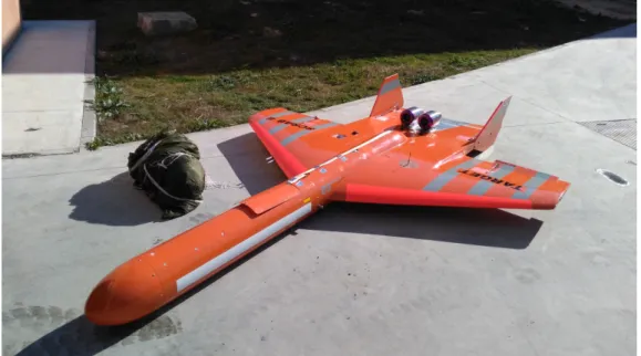
The data to be applied for the purpose of training and evaluating machine learning models was obtained from the logs of a pre-existing real-world network experiment, considering an emerging scenario, carried out in Huelva in 2017. The experiment was performed using an Autonomous Unmanned Vehicle (UAV) performing a flight trajectory and equipped with an antenna, which operated a wireless point-to-point link to a base station. Communication was established between both nodes based on a TCP data flow, and logs of meta information were recorded concerning each packet, containing a set of data-points including the type of packet, the direction of the data flow to which it belonged and the RSSI at the time of reception of each packet. The UAV is additionally equipped with a GPS antenna and with accelerometers, resulting in a separate

Machine Learning Approach for Path Loss Estimation

Figure 3.1: UAV used to capture the dataset during a test flight.

set of records containing an information about the position of the UAV and the angle at regular fixed intervals for the duration of the experiment. Thus, two different sensors, one for network information, and another for positional information, are present on-board the UAV, each resulting in a separate dataset. An illustration of the UAV is given in Figure3.1.

As previously explained, the available data is split in two datasets, one containing information about the network communication between devices, and the other containing information about the position and angle of the UAV. Both datasets are a series of timestamped records with the associated state of the experiment at the given time.

The dataset regarding the network information consists of a tabulation separated set of lines, each consisting of a record of a packet which has been sent or received at the network interface in the UAV. Each record on this dataset is referenced by a timestamp given by the local calendar year, month, day, hour, minute, second and millisecond. The available data for each packet consists of: 1. Type of packet - Either an Acknowledge packet marked by the ACK string, or a data packet

marked by the QDATA string.

2. Source - The MAC address of the source network interface. 3. Destination - The MAC address of the target network interface.

4. RSSI - The Received Signal Strength Indication in dBm, if captured at the destination in-terface, 0 otherwise. It is important to note that the precision of the measurement is to the unit, so this value is discrete, not continuous.

The dataset regarding the UAV position and telemetry consists of a series of comma separated values. Each line of this dataset consists of a sample obtained from the GPS module on-board

Machine Learning Approach for Path Loss Estimation

the UAV. In addition to the standard longitude, altitude and latitude features it also contains the measurements of the angle of the drone in terms of roll, pitch and yaw. The set of samples are annotated with a timestamp called mtime, indicating the amount of seconds elapsed between the start of the experiment and the recording of the GPS datum in question.

3.2

Data Preparation

In order to be able to apply the raw data as described in the previous section to learning a model for the wireless signal strength it is necessary to perform a preprocessing step to wrangle the data into a suitable shape for training, as well as to clean it of invalid or missing values. In very large datasets or unbalanced dataset it may also be necessary to perform sampling in order to reduce the learning step to a computationally tractable problem.

3.2.1 Data Transformation and Cleaning

This section provides an analysis of the data transformation and cleaning operations which were performed to eliminate spurious or incorrect information in each of the two datasets discussed in Section3.1.

The network dataset contains a lot of irrelevant information for the problem at hand. The useful features which were extracted are the timestamp and the RSSI value. The timestamp is converted into elapsed seconds since the beginning of the experiment by fixing a point at which measurements from both sensors have stabilised. Subsequently the data-points which concern transmissions from the UAV to the Base Station were discarded, as no RSSI data is provided for the transmitted packets.

The position and telemetry dataset also contain a number of features with no relevance. From this dataset we extract the measures of longitude, latitude, and altitude, together with the mea-surements of the roll, pitch, and yaw of the UAV. Additionally the timestamp was aligned with the timestamp of the network dataset by referencing the GPS time. This does not eliminate com-pletely the chance of a clock drift, as time elapsed measurements were taken by different clocks. This clock problem could be solved, for instance, by frequently synchronising the system clock with the GPS clock. Nevertheless, this problem is out of the scope of this dissertation and will not be addressed.

3.2.2 Timestamp Interpolation

In analysing and treating the data available, we are faced with the problem that our features are gathered from the output of two different sensors. As explained in Section 3.1 two different sensors are used for gathering network information and positional information. These sensors exhibit different sampling behaviour. In particular the GPS sensor captures position information at a rate of approximately 120 Hz, while the network interface intercepts packet data exactly once per packet received. The consequence of this behaviour is that network datapoint sampling varies

Machine Learning Approach for Path Loss Estimation

0

500

1000

1500

2000

Elapsed Experiment Time (s)

0

2000

4000

6000

8000

10000

12000

14000

16000

18000

Number of Samples

Telemetry Samples

Network Samples

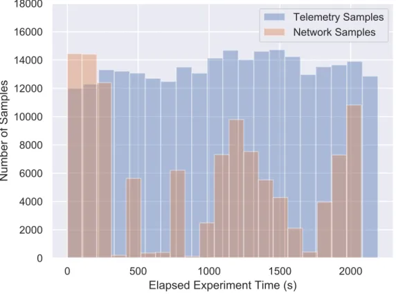
Figure 3.2: Histogram of the samples collected by time, according sensor.

significantly with time, exhibiting periods of high activity and periods where no packet is received and thus no data is available. This difference of sampling frequency between telemetry (hereinafter also called positional information) and network samples is illustrated by Figure3.2.

To resolve this issue there is a need to align the two disjoint datasets into a single dataset [MPP+10]. This unified dataset should contain, for each row, a value consisting of the union of the set of features available in the positional and network datasets. Since there are very reduced chances that a network sample was obtained at the same time as a positional sample, the process of aligning the two datasets is forcefully a lossy one, where the data-points in one of the datasets are interpolated in order to estimate their value at a given point in time where there exists a sample for the other dataset.

As we can observe in Figure3.2 there are significantly more positional information samples than network samples. Furthermore the distribution of the positional samples are much more homogeneous when compared to the network samples, where significant periods of very little to no information are observed, followed by periods of increased activity. Furthermore, the information contained in the positional dataset is much smoother than the information contained in the network dataset, i.e., it is less prone to sudden changes in velocity. From a physical point of view this is due to the largely continuous nature of the movement the UAV describes along its trajectory.

Machine Learning Approach for Path Loss Estimation

Regarding the signal strength at the receiver, it can be modelled as a function of both slow fading or shadowing components, which vary slowly, and fast fading components, both constructive and destructive, which may cause rapid variation of the signal strength. Finally, it is important to notice that the network dataset constitutes the target variable of the modelling problem being tackled, – i.e., the Signal Strength –, while the positional information will merely provide a set of features which will be used to model the problem.

Given the considerations laid out above, it was decided to interpolate the dataset containing positional data-points in order to align it to the network dataset. Consequently, for each packet captured, the position at which the UAV was located and the other positional information will be interpolated from the respective dataset. This process was performed by retrieving, for each network datapoint, the two corresponding positional datapoint whose timestamp were immediately greater and lower compared with its own. The final values for the positional features were then calculated by computing the weighted average by timestamp value of their individual values. This approach preserves the integrity of the signal strength information, but at the same time leads to a heavily unbalanced dataset, with many periods of little to no data-points being available followed by periods of significant sample volume.

3.2.3 Sampling

The unbalanced nature of the aligned dataset means for some positions of the UAV we have a lot of samples providing information about signal strength at that particular point, while other positions have significantly less samples. This overrepresentation of some of the positions and sub-representation of others leads to excessive computational load in processing all the samples.

To solve this problem the dataset was binned by timestamp, with each bin corresponding to samples obtained in a period of one second. Each bin is converted to a single datapoint by finding the mode of the RSSI for each bin and selecting randomly from the set of data-points whose RSSI value equals the mode. The resulting dataset contains one sample for each second of the experiment, except for time periods on which no packets were received, in which case there are no samples.

3.2.4 Normalisation

The features which will be used in the training of the machine learning model have values whose magnitudes are very different, depending on the domain. For example, the altitude feature is rep-resented in meters, and has a maximum magnitude of around 500 meters. Latitude and longitude on the other hand, has a value amplitude of only a few thousandths, due to being represented in degrees according to the standard coordinate system.

Some regression algorithms perform badly when subject to large discrepancies in the scale of the input features. Support Vector Machines, for example, are notoriously reliant on standardi-sation of the data-points being used for training [Kum12]. Others, such as Decision Trees, are

Machine Learning Approach for Path Loss Estimation

Latitude (degrees)

0.64660.6468

0.64700.6472

0.64740.6476

0.1186

0.1184

Longitude (degrees)

0.1182

0.1180

0.1178

0.1176

Altitude (m)

100

200

300

400

500

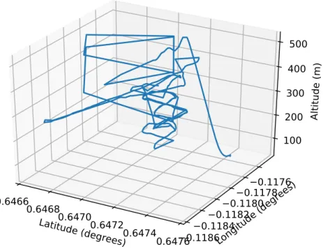
Figure 3.3: Trajectory of the UAV during the experiment, altitude not to scale.

independent on invariant in terms of individual transformations to the value of the features, and as such are not sensitive to data which has not been normalised.

For this dissertation the decision was made to normalize features using the Min-Max normal-isation procedure. This means that for each feature in the input set, the minimum and maximum value were computed. Subsequently each datapoint was rescaled so that the maximum value of the feature is equal to 1 and the minimum value equal to 0. The formula applied for the transformation is given by Equation3.1. valuei= fi− fmin fmax− fmin (3.1)

3.3

Final Dataset

In this section we present the dataset which resulted from the data transformation and cleaning process described in Section3.2. The resulting dataset contains 7 features and a timestamp.

The timestamp is a useful metric to visualize how the UAV’s position changed during the experiment, and was useful to align the two datasets. However, this problem cannot be modelled as a time series problem. While signal strength and path loss changes over time, it does not change

Machine Learning Approach for Path Loss Estimation

Mean St. Dev. Minimum 25% 50% 75% Maximum

lat 0.65 0.00 0.65 0.65 0.65 0.65 0.65 lon -0.12 0.00 -0.12 -0.12 -0.12 -0.12 -0.12 alt 311.94 146.35 1.00 225.00 295.00 480.00 536.00 roll 0.06 0.40 -3.09 -0.03 -0.00 0.09 3.13 pitch 0.06 0.07 -1.23 0.03 0.05 0.07 1.53 yaw -0.12 1.87 -3.14 -1.73 -0.22 1.81 3.14 Table 3.1: Central tendency and dispersion characteristics for the dataset features.

as a consequence of the passing of time. As such the timestamp is not a feature which can be used to train the model. In Figure3.3the trajectory of the UAV for the duration of the experiment is shown.

The features we are left with are the roll, pitch and yaw of the UAV along with its geographical coordinates, namely latitude, longitude and altitude. In Table3.1some of the central tendency and dispersion characteristics of the features are described in more detail.

In order to gain insight into the predictive power any given feature may have, the values of each feature and the corresponding RSSI were plotted and a regression line was fitted, resulting in the series of plots available in Figure3.4. The main conclusions are that the features which most strongly correlate with RSSI are longitude and altitude of the UAV.

3.4

Regressor Evaluation

In the previous sections of this chapter the process to build the dataset and the resulting structure was explained. In this section the usage of the dataset to evaluate models for the prediction of signal strength is described. In particular this section goes over the two different target variables and the various algorithms used to train the model, together with the relevant parameterisation choices and cross-validation results.

In order to compare algorithms and tune hyperparameters1 cross validation is performed in conjunction with an exhaustive search on a subset of the domain of the possible values of all hy-perparameters. This approach allows for the comparison of different machine learning algorithms to the dataset, and can be replicated in other scenarios to help select the best model for the scenario.

3.4.1 Target Variables

The machine learning models described in the next sections are trained to predict a value which represents the path loss according to a spatial location and angle. Two different approaches to modelling this value were taken:

Machine Learning Approach for Path Loss Estimation

Figure 3.4: Linear regression of individual features and RSSI.

1. Direct RSSI Prediction - This approach trains the model to predict the value of the real RSSI observed at each data-point in the training set.

2. Correction of Friis - This approach trains the model to learn the difference between the RSSI predicted by the Friis model and the real RSSI observed at each data-point in the training set. The predicted value in the validation data-points is then given by adding the RSSI value given by the Friis model at that point with the prediction provided by the model.

The error metrics for both of these approaches are addressed in the following sections. 26

Machine Learning Approach for Path Loss Estimation

Mean Absolute Error Median Absolute Error Mean Squared Error

Friis 4.56 3.64 31.42

Two-Ray 6.95 6.14 74.92

Log-Distance (γ=1.8) 9.58 9.24 105.15

Log-Distance (γ=2.2) 11.15 11.11 139.13

Table 3.2: Error metrics for the benchmark models.

3.4.2 Benchmark Metrics

For the purpose of evaluating the accuracy of the predictions of the simulated models, Table3.2 presents the error metrics of three common path loss models, namely the Friis model, the Two-Ray model and the Log-Distance model with a γ value of 1.8 and 2.2. For the Log-Distance model the γ parameter is set based on a scenario such as a corridor where obstructions may cause the signal to be stronger in a particular direction, and on a open field scenario, respectively.

3.4.3 Methodology

In order to avoid overfitting the model to a particular division of the dataset between training and testing data, cross validation was employed. The dataset splits were generated by employing a unshuffled k-fold scheme, with 3 splits being extracted. The decision to employ a unshuffled split derives from the continuous nature of the dataset, where each datapoint is numerically close to those who precede and succeed it in the original dataset ordering. If the dataset was shuffled before being split, each division of the dataset would contain data which would be representative of the entire dataset, leading to an optimistic evaluation of the dataset, as samples taken mere moments before or after those present in the testing dataset would be present in the training data.

After the dataset has been split into partitions a given algorithm is then trained on the aggrega-tion of all the partiaggrega-tions except one. The training process generically consists of feeding the chosen algorithm with a set of hyperparameters, data-points and the corresponding target variables. The outcome of this process is a trained model, as defined by a set of parameters. The partition which is left out from the training process is then used to evaluate the trained model, resulting in one or more metrics which describe the performance of the model for that particular train-test split of the data. The process is then repeated until every partition of the dataset has been used for evalu-ating the model. The metrics are then composed by calculevalu-ating the mean value and the standard deviation for each metric.

The process of training an algorithm can be considered to be the process of setting the pa-rameters of a model according to a training dataset. Hyperpapa-rameters, in contrast with the afore-mentioned parameters, are properties of the learning algorithm which control the process through which the parameters are learned. These values must be set to suit the target problem. In this dissertation the value of the hyperparameters was set by performing a grid search over a range of possible values for each hyperparameter. For each combination of values, the cross validation

Machine Learning Approach for Path Loss Estimation 1 2 3 4 5 6 7 8 9 10 11 12 13 14 15 16 17 18 19

Number of estimators

Mean squared error

max features auto sqrt

Figure 3.5: Grid search for Random Forest hyperparameters.

scheme described above is applied. The hyperparameters which yield the best results according to the employed metric are then selected.

The following sections describe the hyperparameter optimisation and the results of the evalu-ation of two different machine learning algorithms.

3.4.4 Random Forest

The Random Forest algorithm consists of training multiple decision trees from samples of the data, which are drawn with replacement. Each node is split according to the best split for a subset of the features being considered, instead of the entirety of the feature set. The hyperparameters that are analysed are the number of decision trees that compose the forest and the subset of features which are considered for each split. The former hyperparameter is made to vary between 1 and 20, while for the latter the two possibilities are using the entire set of features or using the square root of the cardinality of the set of features. The results of the hyperparameter search are summarized in Figure3.5. The best combination of hyperparameters found was using 17 decision trees and considering the entire set of features.

Evaluation measures were computed using cross-validation both for the direct RSSI prediction and the correction of Friis model. The results are presented in Table3.3. This algorithm appears to perform better when calculating a correction to the Friis model than when directly predicting RSSI values.

Machine Learning Approach for Path Loss Estimation

Direct RSSI Prediction Split 1 Split 2 Split 3 Aggregate Mean Error 2.70 3.09 3.58 3.12+-0.44 Median Error 2.2 -2.5 3.4 -2.7+-0.62 Squared Mean Error 7.29 9.49 12.81 14.59+-3.87 Correction of Friis

Mean Error 2.22 2.93 3.31 2.82+-0.56 Median Error 1.38 2.88 2.90 2.39+-0.58 Squared Mean Error 7.07 12.63 15.77 11.82+-4.41

Table 3.3: Evaluation measures for the Random Forest algorithm.

3.4.5 Adaboost

The Adaboost algorithm was applied by using decision trees with a depth value of 9. The hyper-parameters to set are the loss function with each to train, the learning rate to be applied and the number of estimators to train. The grid search for optimal hyperparameters was performed with the values of the learning rate ranging from 0 to 1, and the number of estimators ranging from 50 to 400. The loss function which is used to calculate the weights of the weak learners can ei-ther be linear, square or exponential. The results of the grid search are summarised in Figure3.6. The combination of hyperparameters found to perform the best from among those searched are an exponential loss function, with a learning rate of 1, 0 and 400 estimators.

Evaluation measures were computed using cross-validation both for the direct RSSI prediction and the correction of Friis model. The results are presented in Table3.4. As can be seen the direct RSSI prediction leads to slightly lower error in prediction when compared to the approach where a correction of the Friis model is targeted.

0.01 0.05 0.1 0.3 1.0 Learning rate 50 100 200 300 400 Number of estimators loss = linear 0.01 0.05 0.1 0.3 1.0 Learning rate loss = square 0.01 0.05 0.1 0.3 1.0 Learning rate loss = exponential 14.0 13.5 13.0 12.5 12.0 11.5 11.0 14.0 13.5 13.0 12.5 12.0 11.5 11.0 14.0 13.5 13.0 12.5 12.0 11.5 11.0

Machine Learning Approach for Path Loss Estimation

Direct RSSI Prediction Split 1 Split 2 Split 3 Aggregate Mean Error 2.33 2.76 2.67 2.59+-0.22 Median Error 1.44 2.07 2.31 1.94+-0.45 Squared Mean Error 11.04 11.61 10.38 11.01+-0.62 Correction of Friis

Mean Error 2.75 2.74 3.26 2.91+-0.30

Median Error 2 3 3 2.67+-0.58

Squared Mean Error 16.85 11.31 15.23 14.46+-2.85 Table 3.4: Evaluation measures for the Adaboost algorithm.

3.4.6 Support Vector Regression

A Support Vector Machine was trained to perform regression on the dataset. The kernel choices which were included in the parameter sweeping process were the linear, radial basis function and polynomial kernels, each kernel corresponding to a different process through which the input data is transformed so that a non-linear boundary can be learned as a regression curve. The hyperpa-rameters to select are the soft-margin parameter known as C and the gamma value. A grid search was performed with C varying between 0.001 and 10 and gamma varying from 0.001 to 1. The re-sults of this grid search process can be seen in Figure3.7. The best combination of parameters that could be found in the grid search was the radial basis function kernel with a soft-margin parameter of 1.0 and a gamma value of 0.1.

Evaluation measures were computed using cross-validation both for the direct RSSI prediction and the correction of Friis model. The results are presented in Table3.4. As can be seen the direct RSSI prediction leads to slightly lower error in prediction when compared to the approach where a correction of the Friis model is targeted.

0.001 0.01 0.1 1.0 Gamma 0.001 0.01 0.1 1.0 10.0 C kernel = linear 0.001 0.01 0.1 1.0 Gamma kernel = rbf 0.001 0.01 0.1 1.0 Gamma kernel = poly 20 18 16 14 12 10 20 18 16 14 12 10 20 18 16 14 12 10

Figure 3.7: Grid search for SVM hyperparameters, with negative square of errors metric.