Abstract— Based on signal measurements carried out in the 5.8 GHz band, which is reserved for unlicensed WiMAX in Brazil, this paper evaluates narrowband and wideband characteristics on the suburban area of Tanguá city in Rio de Janeiro State. Fading statistics, coverage and adjusted prediction model such as Hata-COST 231, SUI and UFPA were used in order to find the model that best fits the measurement data before ultimately determining that the UFPA model proved to be the best one. Temporal dispersion is studied through the delay spread and coherence band calculated from the power delay profiles obtained in the sounded channel.
Index Terms— Delay spread, fading, power delay profile, prediction models.
I. INTRODUCTION
Nowadays, the Brazilian Government develops a program known as digital city which provides
internet access for the population through a WiMAX network with WiFi-enabled CPE´s (Customer
Premises Equipment). Three bands are available for WiMAX systems in Brazil: 2.4, 3.5 and 5.8 GHz.
The last is an unlicensed band, for use in ISM (Instrumentation, Scientific and Medical) systems in
5.725 MHz to 5.850 MHz band, and U-NII (Unlicensed National Information Infrastructure), in the
5.150 MHz to 5.825 MHz band [1] and it was chosen for free internet in those digital cities.
Many articles deal with the signal coverage on 2.4 GHz [2]-[3] and 3.5 GHz [4]-[5] for applying
in WiMAX system. However, the 5.8 GHz band is little explored. A modeling in that band was
already made in an underground mine [3] and in wooded cities of Amazon region [6]. New terrain
proposal for SUI model equations is provided in the 5.8 GHz band based on measurements carried out
in cities of Amazon with some vegetation [7] and it will be used in this work.
It is very important to understand the channel behavior on the signal propagation in the 5.8 GHz
band in environments where the digital cities are implemented. These are suburban ones, in general.
Then, to reach good quality of communication it is necessary to have a complete characterization of
the suburban channel in this band, which is not fully explored in the literature, and this article
provides subsidies for the system planner through the parameters calculated from measurements in
this channel besides on results for searching and simulation. For this, the analysis of the experimental
Channel Characterization in the 5.8GHz
Band in a Suburban Area
Wilyam D. T. Meza, Gláucio. L. Siqueira
Center for Telecommunications Studies – PUC - Rio de Janeiro, Brazil [email protected], [email protected]
Leni J. Matos
signal in a suburban area is made. The chosen frequency was 5.765 GHz and the fading statistics and
signal dispersion are analyzed. Narrowband and wideband parameters are calculated and the signal
coverage and the maximum data transmission rate that can be handled in this environment are
obtained.
In Section II, the setup used for sounding the channel and the characteristics of the environment
are presented. Section III deals with the narrowband characterization, including the small and large
fading statistics, narrowband parameters, path loss and signal coverage to test fitness of three models,
Hata-COST 231, SUI and UFPA, available for this frequency band. In Section IV, the wideband
characterization and parameters as delay spread and coherence band are determined and the
conclusion is given in Section V.
II. MEASUREMENT SETUP AND ENVIRONMENT
Table I presents the devices and equipment used in the sounding. Besides them, a Garmin GPS
GPSmap62 and a laptop with Labview installed are used for picking up the position data and the
samples from the NI data acquisition module, respectively.
TABLE I. TRANSMITTER AND RECEIVER SPECIFICATIONS
Transmission (Tx) Equipments Receiving (Rx) Equipments
Vector Signal Generator Anritsu MG3700A Signature High Performance Signal Analyzer Anritsu MB2781B Power Amplifier Minicircuits ZVE-3W-83 33 dB Low Noise Amplifier ABL0800-12-3315 17 dBi Sectorial Antenna OIW-5817P090V Radome Omni-10 dBi Omnidirectional Antenna
On the transmitter side, Figure 1, the equipment was placed on the top of a building with
coordinates S 22.73619º, W 42.71886º and the antenna was 49 m height.
Fig. 1. Transmission setup with antenna pointing towards the city center.
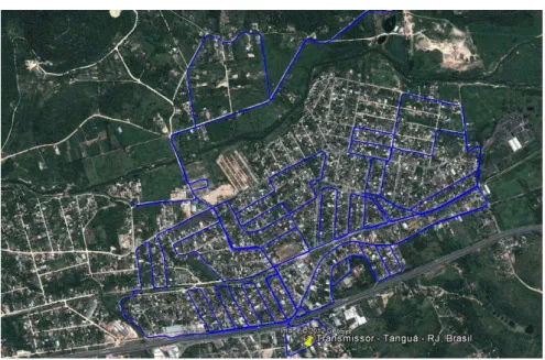
The reception system, Figure 2, was mounted inside a van, with the Rx antenna on its top. The
sounded area was the city of Tanguá, characterized as a suburban one with some vegetation between
characterization, only eight routes have had signal levels above the noise threshold and they are
referred in the Section IV. Figure 3 shows all routes into the city environment. Figure 4 presents the
Route 1 and the Route 2 with graduation color signal level.
Fig. 2. Mobile Measurements Lab (Van).
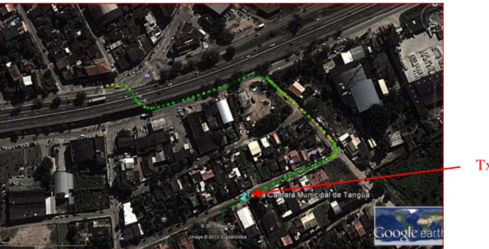
Fig. 3. Aerial view of the measured area and sounded routes. (Source: Google Map)
III. NARROWBAND CHARACTERIZATION
A. Small scale statistics
For searching the narrowband statistics of the channel in the sounded frequency, a 5.765 GHz CW
with 3 dBm level was transmitted to the power amplifier (PA) with a 28 dB gain and the signal was
radiated. Cable and coupling losses were 15 dB aproximately. In an average speed of 30 km/h, the
mobile reception system acquired the signal at a 20 KSPS acquisition rate, saving it for offline
processing.
1. Fading
Sectors of 40 [8] length were taken in order to study the small scale variability of the signal.
The mean signal level in each sector was calculated for studying the large scale variability and then,
the path loss and the signal coverage were determined in the sounded area. Table II presents the
number of sectors taken in the sounded routes and also provides the number of sectors that had the
signal level effectively over the noise threshold and named filtered sectors. It is observed that the
Route 7 had only one sector with signal level above that while the measured signal was totally below
that in the Route 8 and so, this sector was discarded.
TABLE II. ROUTES, SECTORS AND ENVIRONMENT CHARACTERISTICS
Route Sectors/Route Filtered sectors
1 410 410
2 2347 1509
3 295 295
4 1398 764
5 1674 1047
6 935 270
7 1398 1
8 1012 0
9 1569 503
10 1549 1069
11 2295 1267
Even though a 33 dB gain LNA was used in the reception, the environment noise proved high
enough to provide observable sectors on the farthest routes.
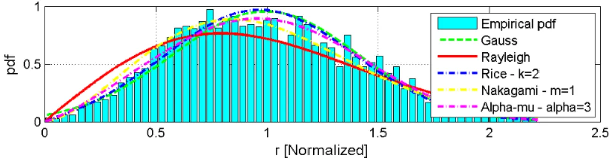
In each sector, probability density functions (p.d.f.) as Gauss [9], Rice [9], Rayleigh [9],
Nakagami [9] and - [10] were adjusted to the measurements in order to identify the one of best
fitting to the environment considered. Figure 5 shows an example for the sector 155 in the Route 1. In
it, Rayleigh is visibly the worst fitted p.d.f. and this occurred in the most of the sectors, as it is
Fig. 5. P.d.f.s fitted to the data in the Sector 155/Route 1.
Among the p.d.f.s used, - showed to have the smallest qui-squared error, in general, adjusting
better to the small scale fading and it was followed by Gauss. The first has shown a good fitting to the
small fading statistics in different channels like that through vegetation [11] in urban park and in
land-air links in an aeronautical channel [12]. Rayleigh p.d.f. showed to be the worst fitting and Rice
fits well in part of the sectors with high values for the k factor, in general. It is remembered that the
Gauss p.d.f. is a limit of the Rice p.d.f. when k factor tends to infinity.
TABLE III. NUMBER OF FILTERED SECTORS THAT FITTED TO THE PDF’S
Route Gauss Rayleigh Rice Nakagami -
1 64 9 63 25 252
2 194 22 95 63 1151
3 33 10 46 17 197
4 58 5 35 14 656
5 129 7 46 30 835
6 69 0 19 0 179
7 0 0 0 0 1
9 73 10 55 53 320
10 146 7 87 33 802
11 131 6 118 35 982
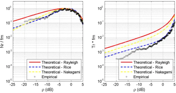
2. LCR and AFD
Starting from the statistics, the level cross rate (LCR) and the average fade duration (AFD) were
calculated for all the filtered sectors and Figure 6 provides an example that shows these parameters
adjusted to the experimental data related to the sector 155 in the Route 1, the same characterized in
Figure 5. It shows that the signal variability is large around the rms value and this is confirmed in
most of the sectors. In this example, the normalized LCR is in the range 0.08 to 1, i.e., the envelope
crosses the rms value in a range from 12.6 to 162 crossings while the normalized AFD is from 3x10⁻⁴
to 0.2, meaning 1.3 to 90 wavelengths for the average fading, both well fitted to Rice channel for this
sector. It is worth observing that the car speed that carried the reception system was 30 km/h in most
Fig.6. LCR and AFD fitted to the data for the Sector 155/Route 1.
B. Large scale statistics
1. Fading
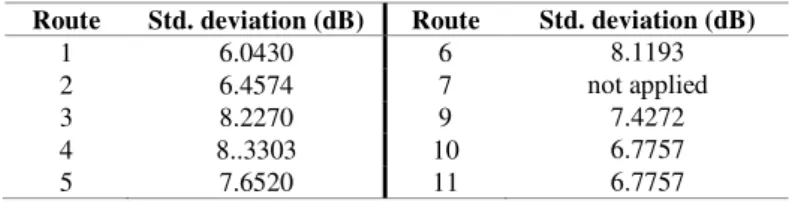
An experimental probability density function (p.d.f.) was adjusted for the large scale variability of
the signal taken as the signal mean in the sectors. Lognormal was the distribution best fitted to it, in
all the routes, and Figure 7 shows an example for the Route 1. In Table IV the standard deviation of
the distribution is presented, which is an important parameter using further in the SUI coverage
prediction model and that varies in the 6.0 to 8.2 dB range [13]. It is observed that Route 7 has only
one sector, so a unique mean and no histogram is possible to plot.
-15 -10 -5 0 5 10 15 20 25
0 0.01 0.02 0.03 0.04 0.05 0.06 0.07 0.08 0.09
Signal Level [dBm]
Empirical PDF Lognormal
TABLE IV. STANDARD DEVIATION OF THE LOGNORMAL P.D.F.
Route Std. deviation (dB) Route Std. deviation (dB)
1 6.0430 6 8.1193
2 6.4574 7 not applied
3 8.2270 9 7.4272
4 8..3303 10 6.7757
5 7.6520 11 6.7757
2. Path loss and coverage
For extracting the path loss from the long term fading, in logarithmic scale of distance as shown
in Figure 8, a straight line was adjusted to it by using the MMSE (Minimum Mean Square Error)
method and then, the attenuation factor could be determined for all routes and they are in Table V.
-0.8 -0.7 -0.6 -0.5 -0.4 -0.3 -0.2 -0.1
-70 -65 -60 -55 -50 -45 -40 -35 -30 -25
Distance from the Tx [km in logaríthm]
S
ig
n
a
l
L
e
ve
l
[d
B
m
]
Best-fit straight loss for the route in the Route 2, n = 3
Fig. 8. Path loss fitted to the large scale fading in the Route 2.
TABLE V. ATENUATION FACTOR FOR THE ROUTES
Rout e
Attenuation factor
() Route
Attenuation factor ()
1 1 6 0
2 3 7 not applied
3 2 9 6
4 3 10 3
5 4 11 3
It is observed that Route 9 presents the highest attenuation factor (equal to 6) due to the terrain
elevation and strong vegetation on that area contributing for the fast decrease of the signal.
For the coverage of the signal, three prediction models were used and they are summarized below.
Extended Hata-COST231
This model is based on Okumura-Hata model with some changes to extend it until 6 GHz
[14]-[15]. The median path loss is calculated as:
a(hm) = [1,1.log f - 0,7].hm - [1,56.log f - 0,8] (2)
where f is the frequency, in MHz; hb is the transmission antenna height, in m; hm is the receiving antenna height, in m; d is the distance between the Tx (Transmitter) and the Rx (Receiver) and Cm is null for suburban area, and 3 dB for urban area. SUI The SUI (Stanford University Interim) model [16] gives the path loss equation and it is based on Erceg model with correction terms for the frequency and the Rx height. The path loss is given by: Aprop = Am + Aprop_f +Aprop_h (3)
Am = [ B + 10( a – bhb + c/hb ) log(d/d0)] + s (4)
B = 20 log(4 d0/) (5)
Aprop_f = 6 log(fMHz/ 2000) (6)
Aprop_h = - 10.8 log(hb/2) (7)
The parameters a, b and c are tabled according to the terrain category. Here, we have considered only b or c, in which: a = 3.6,b = 0.005 and c =20. The variable d is the distance Tx-Rx and d0= 100 m; s is the standard deviation of the lognormal p.d.f. in dB adjusted to the large scale fading; hb is the transmission antenna height, in m, and f is the frequency in MHz. UFPA Starting from measurements carried out in Pará State, Brazil, a model was developed [7] suitable for environment with vegetation characteristic of this State. The final equation for the path loss is: L = K1 log d + K2 log f + K0 (8)
where d is the distance Tx-Rx, in meters; f is the frequency, in MHz; K1 and K2 are parameters obtained with linear least squares; and K0 is a correction factor expressed by: K0 = a – bX (9)
The parameters a and b are adjusted by linear least squares and X is calculated as: X = (H1 + H2)/(0.1 HOB) (10)
where H1and H2 are, respectively, the Tx and Rx antenna height; is the wavelength; and HOB is the
average obstructions height.
Table VI presents a comparison of the error calculated for the fittings in each sounded route.
Models SUI and UFPA have presented a better fit overall and, for a kind of environment like this we
TABLE VI. COMPARISON BETWEEN THE MODELS
Route Model Mean error Std. deviation RMS error
UFPA 2.8751 6.2113 6.8444
1 SUI (B) 17.6366 14.7186 22.9715
Cost231-Hata 32.8722 6.6305 33.5343
UFPA 5.6250 7.0484 9.0178
2 SUI (B) 8.4469 6.8349 10.8658
Cost231-Hata 34.3789 6.8477 35.0543
UFPA 0.0018 8.3148 8.3148
3 SUI (B) 3.7524 9.1287 9.8698
Cost231-Hata 29.0468 8.2525 11.8109
UFPA 6.8107 8.3996 10.8138
4 SUI (B) -0.284 8.4029 8.4077
Cost231-Hata 8.3874 8.3347 11.8244
UFPA 4.0236 8.1957 9.1301
5 SUI (C) 1.1792 7.7339 7.8233
Cost231-Hata 5.9153 7.6564 9.6754
UFPA 3.6085 8.1553 8.9180
6 SUI (C) 0.3050 8.4635 8.4690
Cost231-Hata 5.8182 8.3196 10.1522
UFPA 1.1035 9.2353 9.3010
9 SUI (B) 3.5478 7.5447 8.3372
Cost231-Hata 29.9213 8.9758 31.2386
UFPA 3.4269 7.2828 8.0488
10 SUI (C) -0.3891 9.1154 9.1237
Cost231-Hata 4.1019 7.4522 8.5066
UFPA 2.6408 7.9685 8.3947
11 SUI (B) -4.2234 15.4491 16.0160
Cost231-Hata 30.3843 7.9172 31.3988
Figure 9(a) and Figure 9(b) show examples for Route 4 and Route 5, respectively, which compare
the signal level predicted by the models with those experimental ones. In the SUI model the
environment tested was classified as A (mountain terrain with moderate to high density of trees), B
(plane terrain with moderate to high density of trees) and C (plane terrain with a light density of
trees). In our environment the A category provided the bigger errors.
0.5 0.6 0.7 0.8 0.9 1 1.1 1.2
-120 -110 -100 -90 -80 -70 -60 distance (km) R e c e iv e d p o w e r (d B m ) UFPA Model SUI (B) Model Cost-231 Model Free Espace Model Experimental data
0.4 0.5 0.6 0.7 0.8 0.9 1 1.1
-120 -110 -100 -90 -80 -70 -60 -50 distance (km) R e ce ive d p o w e r (d B m ) UFPA Model SUI (C) Model Cost-231 Model Free Espace Model Experimental data
(a) (b)
IV. WIDEBAND CHARACTERIZATION
In the wideband sounding a 20 MHz OFDM code was generated in Matlab as it is shown in
Figure 10, and sent to the Vector Signal Generator for further radiation through the sectorial antenna.
Receiving the signal with the Signature High Performance Signal Analyzer together the GPS data in a
50 MSPS rate, I and Q components of the signal and the position of the receiver were saved in files
for offline processing. Before starting the GPS (Global Positioning System), its clock was
synchronized to the internal clock of the Signature so that the mobile position and the signal
amplitude were taken at the same time. As the GPS captures the position in 1 second intervals, it was
possible to interpolate position data since the car speed was practically constant. It is important to say
that the sounded environment was the same but the number of routes was different due to the smaller
dynamic range of the wideband measurements.
Fig. 10. OFDM signal used as test signal.
A. Small scale analysis
In wideband analysis the fading is largely seen as the channel behavior along the time and the time
dispersion of the signal, which is characterized by the delay spread and the coherence band. Then, in
small scale they are calculated for each response in time/delay and time/frequency domain,
respectively. From the acquired data and by using the matched filter technique in software, the power
delay profiles (PDPs) were calculated by adequate data processing in order to result the time
dispersion parameters as mean delay, delay spread and coherence band. However, before this
processing, the PDPs were denoised with the WDEN (Wavelet Denoising) technique in order to
identify the valid multipath. The symlet8 functions have already proven good application to the PDPs
and they were used separately to the real and imaginary parts of the PDPs [17]. Table VII provides
TABLE VII. TIME DISPERSION PARAMETERS
It is observed that the delay spread is smaller in the Route 3, which presents LOS to the Tx antenna
and strong signal, as it is seen in Figure 11. In more distant routes it varies in the 0.75 - 1.38 s range
and the vegetation and buildings contribute a lot for the bigger values such as those calculated for
Routes 5 and 6. It is observed in Figure 12 (a), for the Route 1, that the relation between the delay
spread and the coherence bandwidth is not a constant as has found Rappaport [18] in a particular
channel.Then, the transmission rate is variable and with strong predominance until 60 kbps in the
Route 1, as it is observed from Figure 12(b) in which the 90% coherence bandwidth values are
plotted for this route.
Fig. 11. Route 3 and the position of the transmitter.
0 1 2 3 4 5 6 7
0 100 200 300 400 500 600 700 800
Delay Spread (us)
C o h e re n c e B a n d w id th ( K H z )
0 100 200 300 400 500 600 700
0 100 200 300 400 500 600 700 800 Profiles Number C o h e re n c e B a n d w id th ( K H z )
(a) (b)
Fig. 12. Coherence bandwidth in the Route 1 versus: (a) delay spread and (b) profile number. Route Mean delay [µs] Rms delay [µs] Coherence band. [kHz] Number of PDPs
1 0.0924 1.3842 60.8382 693
2 0.0673 0.8025 86.2658 312
3 0.0394 0.3469 100.2463 112
4 0.0591 0.8472 71.4315 440
5 0.0949 1.1558 55.0264 252
6 0.0869 1.1977 57.2796 240
7 0.0780 0.7516 107.8193 142
8 0.0517 0.7519 72.1443 337
B. Large scale analysis
Since the channel stationarity is limited to small scale, when it is desired to determine the
parameters for larger areas it is not possible to do directly from the correlation functions of the
WSSUS channel [9]. So, when dealing with greater distances, the stationarity can only be guaranteed
in pieces through the channel behavior in a small scale and in homogeneous small and adjacent areas.
An analysis that covers each complete route is the calculus of the mean power of the OFDM signal
received along the distance and a comparison of this wideband measurement is made with the
coverage prediction models in order to test the models fitted to the data in the narrowband
characterization of the channel. Table VIII provides the results and it is observed that the fitting error
overcomes those obtained in the narrowband analysis, in general, but the SUI and UFPA prediction
models keep the best adjustment to the experimental values.
TABLE VIII. COMPARISON BETWEEN THE MODELS IN WIDEBAND DATA
Route Model Mean Error Std deviation RMS Error
UFPA 6.995169 5.985115 9.206193
SUI (A) 3.538532 7.703615 8.477434
1 SUI (B) 5.637025 7.430649 9.326875
SUI (C) 8.402019 7.264007 11.10674
HCost231 12.0467 6.498952 13.68793
UFPA 3.90335 7.366751 8.336976
SUI (A) 2.868867 22.32966 22.51319
2 SUI (B) 4.765121 20.87867 21.41554
SUI (C) 7.400022 19.9513 21.27944
HCost231 10.33081 14.98727 18.20285
UFPA 5.29307 7.298524 9.015822
SUI (A) 30.67912 17.01834 35.08322
3 SUI (B) 30.36939 15.87915 34.27021
SUI (C) 31.58525 15.15745 35.03393
HCost231 26.72897 11.42996 29.07029
UFPA 8.328168 5.244329 9.841817
SUI (A) 9.063299 6.806017 11.33425
4 SUI (B) 10.8118 6.507134 12.61895
SUI (C) 13.35165 6.325745 14.77436
HCost231 15.76087 5.520219 16.69964
UFPA 5.091191 6.70981 8.422694
SUI (A) -3.86879 6.561155 7.616842
5 SUI (B) -1.31079 6.547449 6.67737
SUI (C) 1.749784 6.541152 6.771146
HCost231 7.016495 6.541913 9.593114
UFPA 7.921083 6.978229 10.55648
SUI (A) 2.995554 6.879726 7.503597
6 SUI (B) 5.216692 6.859706 8.617972
SUI (C) 8.06058 6.849533 10.57776
HCost231 12.1382 6.831753 13.9287
UFPA 8.017318 6.366559 10.2377
SUI (A) -0.7886 5.326978 5.385033
7 SUI (B) 1.756533 5.30182 5.585222
SUI (C) 4.808836 5.297243 7.154417
HCost231 10.03014 5.432827 11.40698
UFPA 7.849975 6.436107 10.15114
SUI (A) 7.566075 10.18157 12.68503
8 SUI (B) 9.39966 9.610577 13.4431
SUI (C) 11.99425 9.25642 15.15069
V. CONCLUSION
The Brazilian Government develops a program known as Digital City which provides free
internet access for the population, and they are using the unlicensed band of 5 GHz with WiMAX
technology. Therefore, it is important to study the signal coverage on this band to provide channel
data to the operators in order to allow them reach a good coverage planning. Besides this, the
determination of some wideband parameters is important to choose, for example, the appropriate data
transmission rate in this kind of environment.
Brazilian people live majorly in suburban areas for which little, or even none, channel
characterization exists. Hence, this work try to fill this lack of information to help planners to do a
better project. Thus, starting from measurements on the 5.765 GHz band in Tanguá city, Rio de
Janeiro ( a suburban environment), the large scale fading was estimated for several routes and then,
the path loss was determined. In the following step, some prediction models, applied to this band,
were used in order to predict the signal level in this area. By comparing these values with the
experimental ones, among the models used, those that can better predict the signal level in such
environment are: UFPA, SUI and, at last, the Extended Hata-COST231 model. The same occurred
with the OFDM wideband signal. In the routes where the UFPA model was not the best, it presented
an error slightly larger than the SUI model. However, the Extended Hata-COST231 did not fit, in
general, leading to larger errors. It is worth to observe that Tanguá city resembles, in many aspects,
the city where the measurements for generating the UFPA model were carried out. Then, UFPA
model showed to be an appropriate model for predicting the mean signal level in suburban areas with
some kind of vegetation.
From the statistical analysis of fading, it is observed that the channel has behaved as -
distribution in general, followed by gaussian or ricean with high k factor indicating the tendency to
gaussian. The level cross rate (LCR) and average fade duration (AFD) show that the signal variability
is large around the rms value and this is confirmed in most of the sectors. This implies that, although
the signal has a good level, there is the possibility of deep fading, which can fail the communication,
due to the multipath acting not only for enhancing the signal level but also reducing it. Several
techniques help to get round this fading. The use of rake receiver is one of them.
The wideband parameters show that delay spread and coherence bandwidth vary, respectively,
from 0.34 to 1.38 s and 55.03 to 107.82 kHz, indicating that the transmission rate in this channel is
limited to hundreds of kbps and the equalization is necessary for desired larger rates. MIMO
(Multiple In Multiple Out) system and appropriate modulation are techniques which can be used to
increase this rate.
The extensive data array obtained from the measurements permitted to understand the suburban
parameters, providing results that are mainly useful to the planners in order to improve the signal
coverage on this kind of environment and the data transmission rate.
ACKNOWLEDGMENT
To CNPq for the scholarship allowed to one of the authors and to INCT-CSF Project for the financial support.
REFERENCES
[1] ANATEL, “Plano de Atribuições, Destinação e Distribuição de Frequências no Brasil”, pp. 178, 2011.
[2] Alam, D. and Khan, R. H., “Comparative Study of Path Loss Models of WiMAX at 2.5 GHz Frequency Band”, Int. Journal of Future Generation Communication and Networking, vol. 6, N. 2, pp. 11-23,April 2013.
[3] Boutin, M., Affes, S., Despins, C; Denidni, T., ”Statistical Modelling of a Radio Propagation Channel in an Underground Mine at 2.4 and 5.8 GHz”, IEEE Vehicular Technology Conference, 2005, VTC-2005-Spring , vol. 1, pp.
78 – 81, IEEE.
[4] Fonseca, F. J. B. , Dias, P. P., Dal Bello, J. C. R. and Matos, L. J., “Variabilidade e Cobertura de Sinal Rádio Móvel na
Faixa de 3,5 GHz em Ambiente Urbano”, 15º SBMO – Simpósio Brasileiro de Micro-ondas e Optoeletrônica 10º CBMag – Congresso Brasileiro de Eletromagnetismo MOMAG 2012, pp. 1-5, João Pessoa, PB, Brazil.
[5] Shahajahan, M. and Hes-Shafi, A. Q. M. A., Analysis of Propagation Models for WiMAX at 3.5 GHz, PhD Thesis, Blekinge Institute of Technology, pp. 62, Sweden, Sep. 2009.
[6] Castro, B. S. L., Modelo de Propagação para Redes sem Fio Fixas na Banda de 5.8 GHz em Cidades Típicas da Região Amazônica, Dissertação de Mestrado, UFPA, Belém, Brazil, pp. 58, 2010.
[7] Vale, M. F., Gomes, I. R., Castro , B. S. L. , Barros, F. J. B. and Cavalcante, G.P.S., “New Terrain Proposal for SUI Model Equations Based on 5.8 GHz Measurements in Wooded Cities Found in Amazon Region”, 6TH European Conference on Antennas and Propagation Proceedings, pp 1187-1189, 26-30 March 2012, Prague.
[8] Urie, A., “Errors in estimating local average power of multipath signals”, Electronic Letters, vol. 27, issue 4, pp.315-317, Feb 14th,1991.
[9] Parsons, J. D., The Mobile Radio Propagation Channel, John Wiley & Sons, 2nd. Ed., pp. 433, 2000.
[10]Yacoub, M. D., “The − distribution: a general fading distribution, Proc. IEEE Inter. Symp. on Personal, Indoor and Mobile Radio Com., vol. 2, pp. 629–633, Sep 2002.
[11]Leão, E. S., Fonseca, F. J. and Matos, L. J., "Análise Estatística da Variabilidade do Sinal Rádio Móvel Medido em Ambiente de Vegetação", 15º SBMO – Simpósio Brasileiro de Micro-ondas e Optoeletrônica 10º CBMag – Congresso Brasileiro de Eletromagnetismo MOMAG 2012, pp. 1-5, João Pessoa, PB, Brazil.
[12]Paiva, L. S. and Matos, L. J., “Statistical Analysis of the Radiomobile Signal in the 1140 MHz Band of an Aeronautical
Channel”, Microwave & Optoelectronics Conference (IMOC), 2013 SBMO/ IEEE MTT-S International, pp. 1-5, Rio de Janeiro, RJ, Brazil, 4-7 Aug 2013.
[13]Meza, W. D. T., Siqueira, G.L., Santos, M. A. G. and Matos, L. J, “Signal Coverage in a Suburban Area in the 5.8 GHz
Frequency Band”, Microwave & Optoelectronics Conference (IMOC), 2013 SBMO/ IEEE MTT-S International, pp. 1-5, Rio de Janeiro, RJ, Brazil, 4-7 Aug 2013.
[14]Blaunstein, N., Radio Propagation in Cellular Networks, Artech House Publishers, pp. 405, 1999.
[15]Plitsis, G., “Coverage Prediction of New Elements of Systems Beyond 3Gμ The IEEE 802.16 System as a Case Study”, Proc. IEEE VTC 2003-Fall, Vol. 4, pp.2292-2296, Oct 2003.
[16]J.G. Andrews, A. Gosh, and R.Muhamed, Fundamentals of WiMAX: Understanding Broadband Wireless Networking, Prentice Hall, pp. 449, 2007.
[17]Dias, M.H.C. and Siqueira, G.L., “On the Use of Wavelet–Based Denoising to Iimprove Power Delay Profile Estimates from 1.8 GHz Indoor Wideband Measurements”, Wireless Personal Comm., pp.153-175, Springer 2005.