http://dx.doi.org/10.1590/S1982-217020150001000014
SHORT STATIC GPS/GLONASS OBSERVATION
PROCESSING IN THE CONTEXT OF ANTENNA PHASE
CENTER VARIATION PROBLEM
Elaboração de curtas sessões estáticas de observação de GPS/GLONASS no contexto do problema de variação da posição de centro de fase da antena
KAROL DAWIDOWICZ RAFAL KAZMIERCZAK KRZYSZTOF SWIATEK
University of Warmia and Mazury in Olsztyn Faculty of Geodesy and Land Management
Oczapowskiego 1, Olsztyn, Poland
[email protected]; [email protected]; [email protected]
ABSTRACT
TPSHIPER_PLUS antennas) induces a jump (depending on the measurement session) in the vertical component within to 1.3 cm (GPS-only solutions) or within 1.9 cm (GPS/GLONASS solutions).
Keywords: PCV;GPS; GLONASS; ANTEX.
RESUMO
Até agora foram elaborados três métodos de modelagem a variação (de posição) do centro de fase das antenas GNSS (PCV). Por isso e tendo em conta alguns problemas relacionados com a implementação dos modelos absolutos, neste momento podem ser citados três modelos PCV para as antenas dos receptores (relativos, absolutos convertidos e absolutos) e dois modelos para as antenas de satélites (padrão e absolutos). Ademais, analisando ao mesmo tempo as observações de vários sistemas de posicionamento, por exemplo, GPS e GLONASS, podem ser esperadas mais complicações resultantes da estrutura diferenciada dos sinais e diferenças na constelação dos satélites. O objetivo do presente trabalho foi a análise das diferenças da altura, obtidas com base na elaboração de sessões estáticas curtas de medições GPS/GLONASS, resultantes de aplicação de vários modelos de calibração das antenas. A análise foi feita com base em três dias de observações de GNSS, realizadas com três modelos diferentes de receptores e antenas, divididas em sessões de observação de meia hora. Os resultados mostram que a alteração dos modelos relativos de PCV em absolutos pode influenciar significativamente a determinação de altura, particularmente no caso quando os trabalhos exigem alta precisão. O problema é particularmemte visível na elaboração conjunta de observação GPS/GLONASS. Nos estudos realizados, a atualização do modelo de calibração da antena do receptor (usando antenas LEIAT504GG, JAV_GRANT-G3T i TPSHIPER_PLUS), do relativo para o absoluto, causou picos verticais da componente, conforme a sessão de medição, até 1,3 cm (para a solução GPS) ou até 1,9 cm (para a solução GPS / GLONASS).
Palavras-chave: PCV;GPS; GLONASS; ANTEX.
1. INTRODUCTION
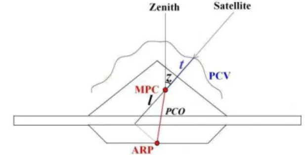
The electrical antenna phase center is the point in space where the GNSS signal is received. However, that point varies depending on the frequency and the direction of the incoming signal, i.e. the elevation angle and azimuth to the satellite. The azimuth is the horizontal angle from true north to the satellite in a clockwise direction. Elevation is the pointing angle from the horizon to the satellite.
To solve the problem, some antenna points must be defined (Figure 1). The first of them is the mean position of the electrical antenna phase center (MPC). Each frequency has a different MPC offset. Next, the antenna reference point (ARP) is
defined by the IGS as the intersection of antenna’s vertical axis of symmetry with
antenna reference point. Finally, the antenna phase center variations (PCV) is the deviation between the positions of the electrical antenna phase center of an individual measurement and the mean electrical antenna phase center.
Figure 1 - GNSS antenna ARP, MPC and PCV point locations.
A review of the antenna phase center variations problem can be found, for example, in Braun et al. (1993), Dawidowicz (2011, 2013), Geiger (1998), Hofmann-Wellenhof et al. (2008), Krueger et al. (2009), Huinca et al. (2012, 2013), Menge et al. (1998), Menge (2003), Montenbruck et al. (2009), Rocken (1992), Schmid et al. (2005), Schmitz et al. (2002), Schupler and Clark (2001), Wanninger (2000, 2009), Völksen (2006).
Spatial relations between ARP, MPC and PCV points are determined by the calibration process and antenna phase center corrections models can then be created and expressed by (DACH et al., 2007):
PCC(a,z) = t(a, z) + PCOe (1)
where:
PCC(a, z) - the total phase center corrections in direction a (azimuth) and z (zenith angle);
PCO - the position of the MPC with respect to the mechanically defined ARP; e - the unit vector in the direction from the receiver ARP to satellite;
t(a, z)- the spherical harmonic function of the phase center variations.
This process involves collecting and processing several hours of GNSS data, and it involves several assumptions about antenna characteristics.
Accurate and consistent modeling of the antenna phase centers continues to be one of the most vexing problems in GNSS analysis. Actually, three main methods have been distinguished to determine GNSS antenna phase center variations:
-absolute field calibrations.
In relative field calibration, the PCV of one antenna is determined relative to another, reference antenna. For this reason, only the differences in the phase center behavior between the two antennas may be computed. (MADER, 1999; ROTHACHER and MADER, 1996). The results for the PCV of the tested antenna are relative to a reference antenna. As per definition, the PCV of this reference antenna are set to zero and the offsets are fixed. The typical reference antenna for the relative field calibration is the AOAD/M_T choke ring antenna. Their average L1 and L2 phase center offsets are defined as 11.0cm and 12.8cm respectively. Because of the influence of site multipath and the insufficient covering of the antenna hemisphere with observations, no azimuth dependence is estimated in these PCV solutions and corrections have a minimum elevation mask of 10 degrees.
In anechoic chamber measurements, an absolute antenna PCV is obtained. The method is based on analyzing how the location of the phase center of an artificial GNSS signal is changed when the antenna, put into an anechoic chamber, is rotated and tilted. (GÖRRES et al., 2006; ROTHACHER, 2001; ZEIMETZ and KUHLMAN, 2008). The main idea is to simulate the different signal directions by rotations of the GPS antenna. The calibration device consists of a fixed transmitter on one end and a remote-controlled positioner carrying the test antenna on the other end of the test chamber. To avoid multipath effects, the calibration measurements are made in anechoic chambers. The positioner rotates the test antenna by small amounts of elevation and azimuth. In this way, it is possible to simulate the different GPS-satellite directions. During calibration, a network analyzer measures the phase shift between the outgoing and incoming signals at each of the simulated satellite positions.
Initially, relative antenna phase center models were used. Later, in 2006, the International GNSS Service (IGS) changed to absolute antenna phase center models. Because there are not yet results of absolute calibrations for all antenna types, absolute models are created for these antennas through the conversion from relative models. Thus, at present we can speak of three models of receiver antennas and two GNSS satellites. For receiver antennas, we have:
- the relative IGS antenna phase center correction model (from relative field calibration),
- the absolute IGS antenna phase center correction model (converted from relative - all the relative antenna offsets and phase center variations have been added to the absolute values for AOAD/M_T antenna),
- the absolute IGS antenna phase center correction model (from absolute field calibration).
For GNSS satellites, there are:
- the standard IGS antenna offset model,
- the absolute antenna phase center correction model.
The many possible available models may introduce some perturbation. Additionally, simultaneously processing observations from different positioning systems, e.g. GPS and GLONASS, we can expect a further complications resulting from the different structure of signals and differences in satellite constellations. As is well known, each GLONASS satellite completes an orbit in approximately 11 hours, 15 minutes, while a GPS satellite completes an orbit in approximately 11 hours, 58 minutes. Another potential difficulty is the fact that different GLONASS satellites transmit signals on different frequencies and, as we know, PCV depend on signal frequency. A review of the GPS/GLONASS observation processing problem can be found, e.g. in Bruyninx (2007), Dodson et al. (1999), Solfa Pinto et al. (2013), Wanninger and Wallstab-Freitag (2007), Weber et al. (2005). In the author’s opinion, however, there is an obvious lack of similar studies connected to the PCV problem.
GLONASS satellites transmit signals using Frequency Division Multiple Access (FDMA) and have 12 allocated radio frequency carriers available in the L1 frequency band and 12 carriers in the L2 band. Each satellite transmits signals at two frequencies, using one assigned radio frequency carrier in the L1 frequency band and one assigned carrier in the L2 frequency band (HOFMANN-WELLENHOF et al., 2008).
estimated PCV from the mixture of observed GLONASS frequencies. Therefore, the calibration is satellite constellation-dependent and is not expected to be as accurate as for the GPS (WÜBBENA et al., 2006).
An alternative PCV modeling has been developed, which allows frequency dependent GLONASS PCV in terms of the individual frequency of the satellites determined. The fundamental assumption of the model is the linearity of PCV changes for GPS/GLONASS and GLONASS/GLONASS frequencies (SCHUPLER and CLARK, 2001). Eventually, it will be common to use GPS PCV for the correction of GLONASS PCV with a lack of better information. However, several issues related to GLONASS PCV are still pressing and important to investigate.
The aim of this paper is to study the height differences in short static GPS/GLONASS observation processing when different calibration models are used. The analysis was done using 3 days of GNSS data, collected with three different receivers and antennas, divided by half-hour observation sessions. In such short
sessions, height changes can be visualized as a result of changes in the satellite’
constellation above the point of measurement. Additionally, when simultaneously processing observations from GPS and GLONASS systems, some complications may arise from the different structure of signals, differences in satellite constellations and problems in GLONASS PCV modeling.
Because studies have shown that the impact of switching from standard IGS antenna offsets to absolute phase center corrections, for the antennas of satellites in a local network (for baselines < 80 km), for height determinations less than ±0.5 mm (CHATAZINIKOAS et al., 2005), the following analysis focuses only on the problem of PCV receiver antennas.
2. METHODOLOGY OF STUDIES
This paper analyses the height differences in GNSS observation processing as a result of switching from relative to absolute receiver antenna calibration models. Both the relative and absolute calibrations models are available on the NGS website (http://www.ngs.noaa.gov/ANTCAL/). All investigations were intended to evaluate
the impact on height determination from the end user’s point of view: the software,
the correction models and processing parameters were the same as any other person would have used.
Topcon Tools v. 6.11 software was chosen for post-processing. In the software it is possible to introduce (define) PCV model by editing the antenna.xml file. This software is an example of a so-called “commercial” software and its main advantage is its simplicity of operation – it only requires the operator to know the principles of GPS observations processing. On the other hand, most of the processing options (e.g. processing frequency, troposphere model or ambiguity resolution strategy) are beyond the possibilities of selection. In Topcon Tools, automatic selection of processing frequency is as follows:
- 0-10 km baselines processing is L1 and L2,
- 30-400 km baselines processing is wide-lane combination.
It is well-known that over very short baselines, higher precision results are obtained using single frequency (L1) differential GPS data than with dual frequency data. This has two reasons. First, ionospheric effects at the two ends of a short baseline are very similar and cancel in differential processing. Second, observational noise of the L3 linear combination is larger by a factor of ~3 than for L1 observations only and also L3 combinations considerably amplify systematic effects due to multipath, antenna phase center offsets and variations, etc. Generally, single-frequency observations (L1) are used for processing baselines not longer than 10-15 km, where the ionospheric delays cancel out during differencing of the observations. The lower cost L1 GPS receivers can provide more precise surveying than more expensive dual frequency receivers over baselines up to 30 km in length (ROCKEN at al., 2000). However, this approach requires the ionospheric delay to be modeled with a high level of precision. Single frequency receivers using such a model can provide better GPS surveying results than dual frequency receivers, even during solar maximum conditions. Generally, when processing longer than 10-15 km baselines, the ionosphere model should be taken into account in order to reduce the residual delays.
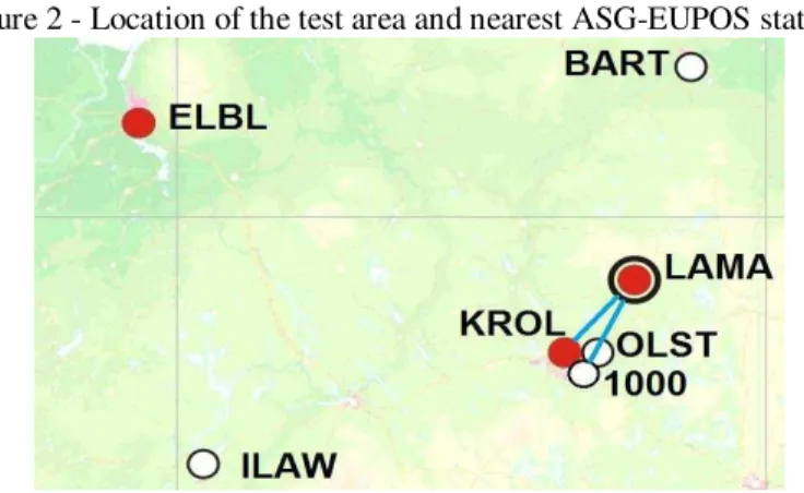
Because we want to use linear combination in observation processing, which causes antenna phase center variations of both frequencies to appear in the final results, suitable point locations had to be selected. We chose the point locations so that the average length of the baselines was about 20 km (Figure 2).
Figure 2 - Location of the test area and nearest ASG-EUPOS stations.
Table 1. Hardware on points selected for testing.
Point name LAMA KROL 1000
Antenna type
LEIAT504GG LEIS
JAV_GRANT-G3T JAVAC
TPSHIPER_PLUS
Point localization
Receiver type
Leica GRX1200GG+GNS
S
JAVAD TRE_G3TH
SIGMA
HIPER PRO
Analyses were based on three-day 24-hour observation sessions carried out from 20-23.11.2012.
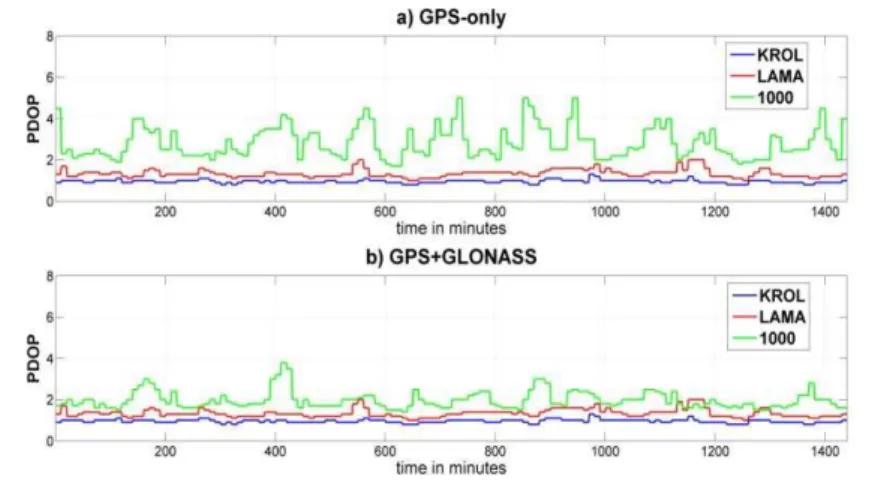
The PDOP coefficient can be seen in the diagram below (Figure 3). The worst situation, as expected, occurred at point 1000, where in some periods the coefficient reaches 5. The PDOP values clearly improve by adding GLONASS observations. In the worst cases, the coefficient does not exceed 4. It should be mentioned that a PDOP value equal to 6 represents a level that marks the minimum appropriate for making surveys and, generally, in such cases GNSS measurements could be used for reliable positioning.
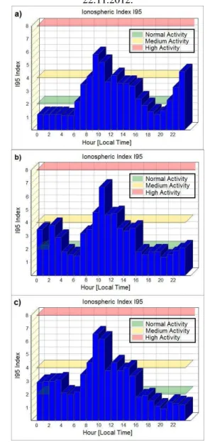
Figure 4 presents the Ionospheric Noise I95 Index for each day of measurement.
Figure 4 - The Ionospheric Noise I95 Index: a) 20.11.2012, b) 21.11.2012, c) 22.11.2012.
The Index 95 values reflect the intensity of ionospheric activity, i.e., the expected influences onto the relative GPS positions. The I95 values are computed from the ionospheric corrections for all satellites at all network stations for the respective hour. The worst 5% of data are rejected.
The following GNSS parameters were assumed for measurements: sampling interval 1s, minimum satellite elevation 10°. 24-hour observations were divided into half-hour sessions and processed in a single-baseline mode using Topcon Tools software in two main strategies:
- using the relative IGS models, - using absolute IGS models.
In each strategy, GPS only and GPS/GLONASS observations were processed. Point locations were chosen so that observations were processed using the so-called
“ionosphere-free linear combination” - L3 (double-frequency observation variant). Using the L3 combination in processing causes the differences in antenna PCV of both frequencies to appear in the final results. Other processing options (tropospheric model, orbits, satellite antenna calibrations, etc.) were identical in all runs.
As is well-known, the main error source in absolute and relative determination of antenna phase center variations is a multipath (WÜBBENA et al. 1996). An environment which is completely unaffected by multipath does not exist. Hence, the antenna phase pattern derived from field procedures is disturbed by a multipath and may create incorrect phase center variations.
The multipath signals are known to repeat at specific sites every mean sidereal day, i.e. every day the same systematics repeat themselves some minutes earlier. This fact has been used in antenna absolute field calibration procedure to greatly reduce the influence of multipath on the determination of phase center variations (WÜBBENA et al. 1996).
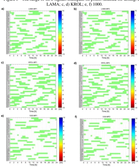
Because knowledge of the multipath at a particular site is important for a number of reasons we present below (Figure 5), colorized maps of high-frequency multipath created on the basis of TEQC report files of single-epoch data.
Figure 5 shows the range of GPS signal multipath errors that can be found on points selected for testing. All signals show minor or no multipath errors. The network station 1000 is, as expected, a slightly more affected station. This agrees very well with the existing obstructions (Table 2) on point 1000.
As expected, the multipath effects are highly correlated with the horizon masks. Generally, only for GPS signals arriving from a low elevation (the appearance and disappearance of satellites) the multipath effects are slightly larger. This can be seen clearly in the multipath detection map (Figure 5).
Figure 5 - The range of GPS signals multipath on points selected for testing: a, b) LAMA; c, d) KROL; e, f) 1000.
The selected measurement antennas are characterized by differences between their phase characteristics and the changes in these characteristics for subsequent types of calibration. A comparison of the antenna phase characteristics on the measured baselines is shown in figures 6-8. The locations of MPC over ARP (“up”
offset) for L1 and L2 frequencies for these antennas obtained from chosen calibration methods are presented in Table 2.
comparison was made in antenna pairs: an antenna on a fixed point and an antenna on an unknown point.
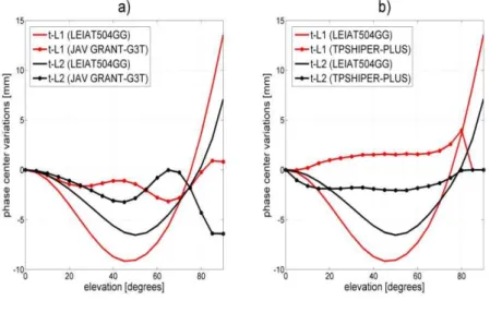
Figure 6 - IGS relative elevation dependent PCV: a) for antenna pair LEIAT504GG and JAV_GRANT-G3T; b) for antenna pair LEIAT504GG and TPSHIPER_PLUS.
Figure 7 - IGS absolute elevation dependent PCV for GPS: a) for antenna pair LEIAT504GG and JAV_GRANT-G3T; b) for antenna pair LEIAT504GG and
Figure 8 - IGS absolute elevation dependent PCV for GLONASS: a) for antenna pair LEIAT504GG and JAV_GRANT-G3T; b) for antenna pair LEIAT504GG and
TPSHIPER_PLUS.
Table 2. The locations of MPC over ARP for antennas used in measurements (mm) Calibration model Locations of MPC over ARP
LEIAT504GG
JAV_GRANT-G3T
TPSHIPER_PLUS
L1 L2 L1 L2 L1 L2
Relative IGS 107.4 126.2 69.4 60.6 105.9 97.1 Absolute IGS 89.6 119.6 50.3 46.8 87.1 89.2
It is clear that the selected antennas have different profiles. Generally, the greatest difference was observed for medium zenith angles (from 30° to 60°), and for the L2 frequency, additionally, for large zenith angles (more than 70°). The maximum difference for the same frequency exceeded over 10 mm. These differences are also visible in comparing PCV characteristics for the same antenna, obtained from different calibration procedures – the maximum differences for the same frequency are up to 10 mm. Clear differences were also found between offsets obtained using the relative and absolute calibration methods. Comparing absolute elevation dependent PCV for GPS and GLONASS signals, there are only small 2-3 mm differences visible.
absolute-converted PCV model available (igs08.atx) without GLONASS PCV corrections. This was also the case in adopting GPS PCV corrections for GLONASS signals in post-processing. Figure 8 presents antenna GPS PCV corrections for TPSHIPER_PLUS.
3.RESULTS AND ANALYSIS
This paper presents the height differences obtained in short baseline GPS/GLONASS observation processing when different calibration models are used. The analysis was done using 3 days of GNSS data, collected with three different receivers and antennas, divided by half-hour observation sessions.
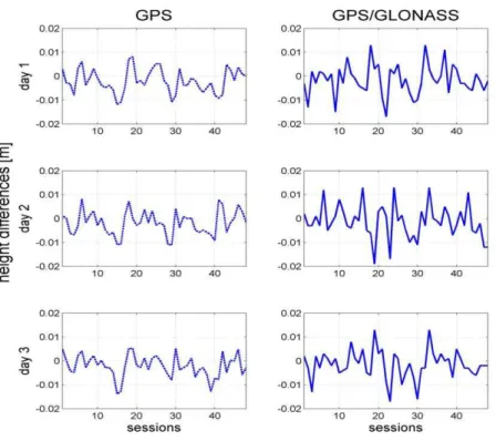
The baseline results obtained with the LEIAT504GG and JAV_GRANT G3T antennas (height differences for previously-mentioned processing strategies, on the JAV_GRANT-G3T antenna point) are presented in Table 3 and Figure 9. The figure shows the height differences obtained from the processing of GNSS observations using absolute and relative field calibration models (absolute – relative). Table 3 shows a summary of the height differences obtained for the baseline.
Table 3 - Summary of height differences obtained for points with the JAV_GRANT-G3T antenna (m).
Day of observations
Height differences for GPS solutions
Height differences for GPS/GLONASS solutions Max. Min. Average Max. Min. Average Day 1 0.0052 -0.0118 -0.0032 0.0128 -0.0166 -0.0024 Day 2 0.0058 -0.0110 -0.0032 0.0141 -0.0172 -0.0039 Day 3 0.0052 -0.0128 -0.0029 0.0133 -0.0174 -0.0033
In analyzing the results obtained for the baseline with LEIAT504GG and JAV_GRANT G3T antennas, it can be seen that the height differences for the GPS-only solutions are within 1.3 cm. Significantly larger differences were obtained for processing done using GPS/GLONASS observations. In comparing the height differences obtained between the results using the absolute and relative calibrations models it is clear that for some solutions its size reaches 1.9 cm. Additionally, for GPS-only solutions there was a 12-hour repeatability of the results, although for GPS/GLONASS it is hard to find a similar behavior.
Figure 9 - The results of processing half hour sessions for baseline with LEIAT504GG and JAV_GRANT-G3T antennas.
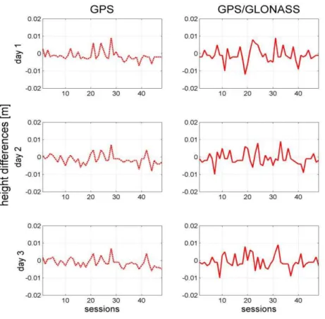
Similar results are presented below for LEIAT504GG and TPSHIPER_PLUS antennas. Figure 10 shows the height differences obtained from the processing of GNSS observations using absolute and relative field calibration models. Table 4 shows a summary of the height differences obtained for the baseline.
Table 4 - Summary of height differences obtained for points with the TPSHIPER_PLUS antenna.
Day of observations
Height differences for GPS solutions
Figure 10 - The results of processing half hour sessions for baseline with LEIAT504GG and TPSHIPER_PLUS antennas.
In comparing the minimum, maximum and average height differences for GPS-only and GPS/GLONASS solutions (Table 4) as before, switching between calibration models more strongly affected GPS/GLONASS results.
Generally, it can be concluded that GPS-only results are comparable to results obtained in other studies (DAWIDOWICZ, 2013; CHATZINIKIOS et al., 2009; FALKO et al., 1998; VÖLKSEN, 2006 ). There is a lack of similar studies on GPS/GLONASS observation processing. Both the large jump in the vertical component and the non-repeatability of GPS/GLONASS results, in the author’s
opinion, is worth further study.
Finally, it should be noted that the obtained height differences are the result of switching from the relative to the absolute PCV model for two pairs of antennas – for other antennas, the results may differ.
4. CONCLUSIONS
In this study, the height differences caused by switching between relative and absolute calibration models in GPS-only and GPS/GLONASS observation processing were compared. The advantage of the absolute approach is clear. Unfortunately, to date, not all antennas have absolute calibration models .
The update of receiver antenna calibrations from relative to absolute in our study (using LEIAT504GG, JAV_GRANT-G3T and TPSHIPER_PLUS antennas) induces a jump (depending on the measurement session) in the vertical component within to 1.3 cm (GPS-only solutions) or within 1.9 cm (GPS/GLONASS solutions). These jumps are relevant for many high accuracy applications.
These jumps are mainly caused by changes in the satellite constellation above the measured points (directions of signals). However, some effects could also be caused by changes in measurement conditions, e.g. ionospheric and tropospheric delay.
Additionally, for GPS/GLONASS observation processing, two trends were noted. Height differences, obtained from the comparison results using absolute and relative antenna PCV models, are significantly larger for GPS/GLONASS solutions. Additionally, the non-repeatability of GPS/GLONASS results is clearly visible. This may result from differences in satellite constellations and the different structure of signals - GLONASS satellites transmit signals on different frequencies and, as we know, PCV depends on signal frequency.
In the author’s opinion, these problems need further investigation.
REFERENCES
BRUNINX, C. Comparing GPS-only with GPS+GLONASS positioning in a regional permanent GNSS network. GPS Solutions,v. 11(2), p. 97-106, 2007. BRAUN, J.; ROCKEN, C.; MEERTENS, C.M.; JOHANSON, J. GPS antenna
mixing and phase center corrections. Eos Trans. AGU, Fall Meeting
CHATAZINIKOS, M.; FOTIOU, A.; PIKRADIS, C. The effects of the receiver and satellite antenna phase center models on local and regional GPS networks.
Proceedings of the International Symposium: Modern technologies, educations
and professional practice in geodesy and relative fields, 5-6 November, Sofia,
2009.
DACH, R.; HUGENTOLBER, U.; FRIDEZ, P.; MEINDL, M. Bernese GPS Software Version 5.0.Astronomical Institute, University of Bern, p. 327-346, 2007.
DAWIDOWICZ, K.; ŚWIĄTEK K. Some aspects of GPS observation elaboration for heights appointment requirements, Proceedings of the 7th International
Conference ENVIROMENTAL ENGINEERING, Selected papers volume III: p.
1300-1304, 2008.
DAWIDOWICZ, K. Comparison of using relative and absolute PCV corrections in short baseline GNSS observation processing. Artificial Satellites, v. 46, p. 19-31, 2011.
DAWIDOWICZ, K. Impact of different GNSS antenna calibration models on height determination in the ASG-EUPOS network – a case study. Survey
Review, v. 45(332), p. 386-394, 2013.
DODSON, A.H.; MOORE, T.; BAKER, F.D.; SWANN, J.W. Hybrid GPS+GLONASS. GPS Solutions, v. 3(1), p. 32-41, 1999.
FALKO, M.; SEEBER, G.; VÖLKSEN, CH.; WÜBBENA, G.; SCHMITZ, M. Results of Absolute Field Calibration of GPS Antenna PCV.Proceedings of the 11th International Technical Meeting of the Satellite Division of the Institute of
Navigation, 15-18 September, Nashville, TN; UNITED STATES, p. 31-38,
1998.
GEIGER, A. Modeling of Phase Center Variation and its Influence on GPS Positioning.Proceedings of the International GPS-WorkshopDarmstadt:
GPS-Techniques Applied to Geodesy and Surveying, 10-13 April 1998, Darmstad, v.
19, p. 210-222, 1998.
GÖRRES, B.; CAMPBELL, M.; BECKER, M.; SIEMES, M. Absolute calibration of GPS antennas: Laboratory results and comparison with field and robot techniques, GPS solutions, v. 10, p. 136-145, 2006.
HOFMANN-WELLENHOF, B.; LICHTENEGGER, H.; WASLE, E. GNSS – Global Navigation Satellite Systems. Springer-Verlag Wien, Austria, 2008. HUINCA S.C.M.; KRUEGER, C.P.; MAYER, M.; KNÖPFLER, A.; HECK, B.
First Results of Relative Field Calibration of a GPS Antenna at BCAL/UFPR (Baseline Calibration Stations for GNSS Antenna at UFPR/Brazil), International Association of Geodesy Symposia 136 “Geodesy for Planet Earth”, p. 739 – 744, 2012.
HUINCA S.C.M.; KRUEGER, C.P; HECK, B.; MAYER, M.; KNÖPFLER, A. BCAL/UFPR - The GNSS Antenna Calibration Service of Latin America.
International Association of Geodesy Scientific Assembly 2013, 1-6 September,
KRUEGER, C.P.; FREIBERGER, J.; HECK, B.; MAYER, M.; KNÖPFLER, A.; SCHÄFER B. Establishing a GNSS Receiver Antenna Calibration Field in the Framework of PROBRAL, International Association of Geodesy Symposia
“Observing our Changing Earth”, p. 701- 707, 2009.
MADER, G.L. GPS Antenna Calibration at the National Geodetic Survey. GPS Solutions, v. 13(1), p. 50-58, 1999.
Magellan Corporation Ashtech Precision Products: Ashtech Solutions Tutorial. Printed in USA, 82 pages, 1999.
Magellan Navigation Inc.: GNSS Solutions Reference Manual. Printed in USA. 472 pages, 2008.
MENGE, F.; SEEBER, G.; VÖLKSEN, C. WÜBBENA, G.; SCHMITZ, M. Results of absolute field calibration of GPS antenna PCV. In: Proceedings of the 11th International Technical Meeting of the Satellite Division of the Institute of
Navigation ION GPS-98, September 15-18, Nashville, Tennessee, 1998.
MENGE, F. Zur Kalibrierung der Phasenzentrumsvariationen von GPS Antennen für die hochpräzise Positionsbestimmung. 198 f. genehmigte Dissertation.
Hannover 2003.
MONTENBRUCK, O.; GARCIA-FERNANDEZ, M.; YOKE, Y.; SCHÖN, S.; JÄGGI, A. Antenna Phase Center Calibration for Precise Positioning of LEO Satellites., GPS Solutions, v. 13 (1), p. 23-34, 2009.
ROTHACHER, M. Comparison of Absolute and Relative Antenna Phase Center Variations. GPS Solutions, v. 4, p. 55-60, 2001.
ROTHACHER, M.; MADER, G. Combination of antenna phase center offsets and variation: antenna calibration set IGS_01. http://ubeclu.unibe.ch, 1996.
ROCKEN, C. GPS antenna mixing problems. UNAVACO Memo, 12 November, 1992.
ROCKEN, C.; JOHNSON, JM.; BRAUN, JJ.; KAWAWA, H.; HATANAKA, Y.; IMAKIIE T. Improving GPS surveying with modeled ionospheric corrections.
Geophysical Research Letters, v. 27 (23), p. 3821–3824, 2000.
SCHMID, R.; ROTHACHER, M.; THALLER, D.; STEIGENBERGER, P. Absolute phase center corrections of satellite and receiver antennas. GPS Solutions, v. 9, p. 283-293, 2005.
SCHMITZ, M.; WÜBBENA, G.; BOETTCHER, G. Tests of phase center variations of various GPS antennas, and some results. GPS Solutions, v. 6, p. 18-27, 2002.
SCHUPLER, B.R.; CLARK, T.A. How Different Antennas Affect the GPS Observable. GPS World , November/December, p.32-36, 1991.
SCHUPLER, B.R.; CLARK, T.A. Characterizing the Behavior of Geodetic GPS Antennas. GPS World, February, p. 48-55, 2001.
SOLFA PINTO, M.; DE OLIVEIRA CAMARGO P.; GALERA MONICO J. F. Influence of combination of GPS and GLONASS data in georeferencing of rural properties, Boletim de Ciências Geodésicas, v.19(1), p. 135-152, 2013. Topcon Positioning System: Topcon Tools User’s Guide. Topcon Positioning
WANNINGER, L.; MAY, M. Carrier Phase Multipath Calibration of GPS Reference Stations In: Proceedings of ION GPS2000, Salte Lake City, UT, p. 132–144, 2000.
WANNINGER, L.; WALLSTAB-FREITAG, S. Combined processing of GPS, GLONASS, and SBAS code phase and carrier phase measurements. In:
Proceedings of ION GNSS 2007, p. 866–875, 2007.
WANNINGER, L. Corrections of apparent position shifts caused by GNSS antenna changes, GPS Solutions, v. 13(2), p. 133 – 139, 2009.
WEBER, R.; SLATER, J.A., FRAGNER, E., GLOTOV, V.; HABRICH, H.; ROMERO, I,; SCHAER, S. Precise GLONASS Orbit Determination within the IGS/IGLOS Pilot Project. Advances in Space Research, v. 36, p. 369-375, 2005.
VÖLKSEN, CH. The Impact of different GPS Antenna Calibration Models on the EUREF Permanent Network. Report on the Symposium of the IAG
Sub-commission for Europe (EUREF), Frankfurt/Main, p. 73-78, 2006.
WÜBBENA, G.; MENGE, F.; SCHMITZ, M.; SEEBER, G.; VOLKSEN CH. A New Approach for Field Calibration of Absolute Antenna Phase Center Variations. Proceedings of the 9th International Technical Meeting of the
Satellite Division of The Institute of Navigation (ION GPS 1996), September 17
- 20, 1996.
WÜBBENA, G.; SCHMITZ, M.; MENGE, F.; BÖDER, V.; SEEBER G. Automated Absolute Field Calibration of GPS Antennas in Real-Time, In: Proceedings of the 13th International Technical Meeting of the Satellite Division of the Institute of Navigation ION GPS 2000, September 19-22, Salt Lake City, Utah, 2000.
WÜBBENA, G.; SCHMITZ, M.; BOETTCHER, G.; SCHUMANN, CH. Absolute GNSS Antenna Calibration with a Robot: Repeatability of Phase Variations, Calibration of GLONASS and Determination of Carrier-to-Noise Pattern.
Submitted to the Proceedings of the IGS Workshop: Perspectives and Visions
for 2010 and beyond, 8-12 May 2006, Darmstadt, Germany, 2006.
ZEIMETZ, P.; KUHLMAN, H. On the Accuracy of Absolute GNSS Antenna Calibration and the Conception of a New Anechoic Chamber. FIG Working
Week 2008, 14-19 June 2008, Stockholm, Sweden, 2008.