Abstract
This study proposes a new pure numerical way to model mass / spring / damper devices to control the vibration of truss struc-tures developing large displacements. It avoids the solution of local differential equations present in traditional convolution approaches to solve viscoelasticity. The structure is modeled by the geometri-cally exact Finite Element Method based on positions. The intro-duction of the device's mass is made by means of Lagrange multi-pliers that imposes its movement along the straight line of a finite element. A pure numerical Kelvin/Voigt like rheological model capable of nonlinear large deformations is originally proposed here. It is numerically solved along time to accomplish the damping parameters of the device. Examples are solved to validate the formulation and to show the practical possibilities of the proposed technique
Keywords
Nonlinear dynamics, truss structures, vibration control, large strain, Kelvin/Voigt rheology.
Kelvin Viscoelasticity and Lagrange Multipliers Applied
to the Simulation of Nonlinear Structural Vibration Control
1 INTRODUCTION
The development of new structural materials with high strength / density ratio leads to the design of structures increasingly lightweight and slender. This type of structure generally develops a level of displacement amplitude greater than those capable of being analyzed by linear models. Further-more, analysis of machines and mechanisms, or civil structures subject to seismic actions, are highly important problems for which the nonlinear dynamic analysis is imperative. Regarding these sub-jects one may consult the works of Sugiyama et al. (2003), Bauchau and Bottasso (2001), Lee et al. (2008), Norton (2011), Spencer Jr and Nagarajaiah (2003), Ramallo (2002) and Moeindarbar and Tagikhany (2014). Thus it is necessary to develop and utilize geometrically accurate nonlinear for-mulations that consider the equilibrium analysis, or motion, at the current configuration of the
Raphael Henrique Madeira a Humberto Breves Coda b
a Departamento de Engenharia de
Estru-turas, Escola de Engenharia de São Car-los, Universidade de São Paulo, Av. Tra-balhador Sãocarlense, 400, CEP 13566-590, [email protected]
b Departamento de Engenharia de
Estru-turas, Escola de Engenharia de São Car-los, Universidade de São Paulo, Av. Tra-balhador Sãocarlense, 400, CEP 13566-590, [email protected]
http://dx.doi.org/10.1590/1679-78252624
structure. In particular, the formulations based on the Finite Element Method are very accepted for solving this kind of problem. Updated Lagrangian and co-rotational formulations can be seen, for example, in Bathe et al (1975), Simo and Vu-Quoc (1986), Armero (2006), Jelenic and Crisfield (2001) and Yoo et al. (2007). Total Lagrangian formulations based on positions and unconstrained vectors can be seen in Coda et al. (2013), Reis and Coda (2014) and Coda and Paccola (2008). The sole advantage of updated Lagrangian and co-rotational formulations is that they are extensions of linear formulations and, as a consequence, various well known literature solutions can be used to improve results. This advantage is also a disadvantage as in updated formulations finite rotations must be linearized and the current stress must be updated using the Kirchhoff-Jaumann formulae, while for the above mentioned total Lagrangian formulation none of these tricks are necessary.
Many lightweight structures, responsible for mechanical support of the designed object, consist of structural elements loaded predominantly by normal force. This kind of structure is usually called truss (Greco et al. (2006)). The finite element used to model trusses do not include bending stiffness bringing difficulties for modeling vibration control devices of the type mass / spring / damper in nonlinear analysis. In practice, this type of device has a mass which must slide over a surface (over a finite element) and its contact force is orthogonal to the member, resulting in bend-ing stresses. Moreover, the dampers used in such devices can be represented by viscous constitutive models that, associated with their stiffness, result in viscoelastic models similar to the Kelvin/Voigt one. The treatment of these linear and nonlinear viscoelastic formulations is usually done by more or less complicated traditional convolution techniques or decaying functions as explained by Le-maitre and Chaboche (1990), LeLe-maitre (2001), Lima et al. (2015), Holzapfel (1996), Simo (1987), Huber and Tsakmakis (2000) and Petiteau et al (2013) used or not in vibration control (Marko et al. (2006) and Clough and Penzien (1985)). There are no significant differences regarding the tradi-tional rheological viscoelastic approach of materials in all consulted bibliography. They use the same procedure, convolution, to solve different viscous materials, developing small or large strains.
In this study, it is presented: (i) a Total Lagrangian truss finite element for geometric nonlinear dynamic modeling of two- and three-dimensional structures. (ii) a technique based on Lagrange multipliers for the consideration of passive mass / spring / damper vibration control mechanisms and (iii) an innovative approach to the consideration of viscous damping in the form of the rheolog-ical model of Kelvin/Voigt adapted to the Green nonlinear strain derived from linear applications (Mesquita and Coda (2002), Mesquita and Coda (2003) and Mesquita and Coda (2007)).
The main contribution of this study is item (iii) that introduces a pure numerical way to con-sider viscous material behavior in dynamic or static applications. The proposed formulation avoids the analytical solution of time differential equations for each considered material law and the use of its solution as a residual in a convolution technique. Therefore, differently from the existent formu-lations, the proposed strategy can be easily extended to be used in any viscoelastic constitutive rela-tion, linear or not.
making use of Lagrange multipliers. Representative examples are presented in section 5 to validate the proposed formulation and describing its practical possibilities. Conclusions are presented in sec-tion 6.
2 TOTAL MECHANICAL ENERGY AND STATIONARY PRINCIPLE
The principle of stationary energy indicates that the equilibrium of mechanical systems occurs when the variation of the total mechanical energy is zero. When it comes to dynamic applications, using the D'Alambert principle, the dynamic equilibrium is meant the equation of motion.
The principle of stationarity is usually employed when dissipative forces do not appear because, in this case, system energy level falls continuously over time. However, it is possible to apply the principle of stationarity considering a larger energy system than the system studied, in which the dissipated energy is part of it. Thus, the total mechanical energy to be considered in this study is written as.
U
K
P
Q
(1)Where U is the strain energy K is the kinetic energy, P is the potential of external forces (con-sidered conservative) and Q is the dissipative potential resulting from the considered damping de-vice. The total energy variation can be expressed as:
0
U
K
P
Q
(2)In truss structure analysis it is usual to consider external forces applied to the nodes of the structure, as well as concentrated mass at nodes, otherwise it would be admitting the existence of bending stresses in structural elements, which is not possible by the mechanical definition of truss elements. Thus, the primary variables of the problem are nodal positions.
Therefore, to establish the adopted finite element formulation it is necessary to write equation (2) as a function of nodal position of the structure.
2.1 Kinetic Energy and External Forces Potential
Using index notation, the potential of external applied forces is given by:
i i
P
F Y
(3)in which the external forces
F
i are considered conservative, i.e., they do not depend on positions. In equation (3)
i
represents direction and truss nodes on which the forces are applied or po-sitions measured. The variation of external forces potential, taken in relation to nodal popo-sitions, is written as:
i i
ij i j i ij j i i
j j
F Y
Y
P
Y
F
Y
F
Y
F
Y
Y
Y
(4)One writes the kinetic energy for the analyzed structure as:
0
0 0
1
1
2
fenfe
i i V
fe
K
y y dV
(5)where the over dot indicates time derivative, fe stands for finite element and nfe is the number of
finite elements. To write the variation of kinetic energy one applies the principle of conservation of mass, i.e.:
0 0 0
1 1 1
1
2
fe fe fenfe nfe nfe
i i i i i i
V V V
fe fe fe
K
d
K
dt
y y dVdt
y y dt dV
y y dV
dt
dt
(6)Remembering that, for trusses, mass is considered concentrated at nodes, one writes:
( )
i i
K
M
Y
Y
(7)in which, M is the mass corresponding to node , calculated as half the sum of the masses
corre-sponding to finite elements connected to the node plus, when needed, the concentrated masses ex-istent in the structure.
2.2 Strain Energy
In the previous item the mechanical energies that depend directly on the position of the nodes of the structure are presented. This section shows the strain energy that depends indirectly on the nodal positions. Firstly, one defines the adopted strain measure and its dependence of positions. Then the specific strain energy is presented as a function of strain and the dependence of nodal position becomes clear.
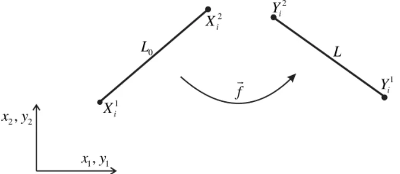
Figure 1 shows a truss element before and after the change of position or movement. The initial position of the element is defined by the initial position of nodes, i.e., Xi
in which 1, 2,3 i
repre-sents direction and nodes. The current position is defined by the unknown variables, i.e., the current nodal positions called Yi
. First of all it is important to inform that unknown nodal
posi-tions are determined by a predictor corrector numerical algorithm. Therefore, the following expres-sions are written containing these unknowns, but trial values are always known.
0
L L
f
1, 1 x y 2, 2
x y
1 i X
2 i X
2 i Y
1 i Y
The initial and current lengths L0 and L are calculated by:
2
2
22 2 1 2 1 2 1
0 1 1 2 2 3 3
L
X
X
X
X
X
X
(8)
2
2
22 2 1 2 1 2 1
1 1 2 2 3 3
L
Y
Y
Y
Y
Y
Y
(9)The one-dimensional Green-Lagrange strain is chosen to describe the material behavior, i.e.:
2
2 0
1 L
E
1
2 L
(10)From the calculated Green's strain one can choose any Lagrangian constitutive relation to rep-resent the material. In this work the uniaxial constitutive relation of Saint-Venant-Kirchhoff is cho-sen and is expressed by the specific strain energy and its derivative with respect to the Green strain as
2
1
u
E
2
E
.
u
S
E
E
E
(11)
in which
E
is the elastic modulus that coincides with the Young modulus for infinitesimal (orsmall) strains and S is the longitudinal second Piola-Kirchhoff stress related to the Cauchy stress by
L L/ 0
.S as described by Ogden (1984) and Bonet et al. (2000).Integrating the specific strain energy on the initial volume of the bar (Lagrangian quantities) one finds the accumulated strain energy on a finite element and structure, such as:
fe 0
fe
2 fe 2
fe V 0 0 0 0
1
1
U
udV
E
V
E
A L
2
2
E
E
and1
nfe fe fe
U
U
(12)It is worth noting that all quantities are assumed to be constant along the bar, facilitating the integration process. It is obvious that expression (12) depends on the current positions of the nodes of the structure. Then, one calculates the variation of strain energy regarding positions as:
1
fe nfe
i i
fe
i i
U
U
U
Y
Y
Y
Y
(13)Using expression (12) one writes,
2
0 0 0 0 0 0
1
.
2
fe
fe fe fe
i i i i
U
E
E
E
A L
E A L
S A L
Y
Y
Y
Y
E
E
(14)
2 1
2 2 1
2 2 1
21 1 2 2 3 3
2 0
Y
Y
Y
Y
Y
Y
1
E
1
2
L
(15)
2 1
i i
2
i 0
E
( 1 )
Y
Y
Y
L
(16)Substituting equation (16) into (14) and using the energy conjugate definition (Ogden (1984) and Bonet et al. (2000)), that is, the derivative of strain energy regarding position (or displacement) results internal force, one writes:
2 1
0 0 2
int
0
( 1)
fe fe
i i i
F
E A L
Y
Y
L
E
(17)
Equation (17) represents the contribution of an element for the total internal force of the ana-lyzed structure. The internal forces are calculated for all finite elements and are combined into a single vector of internal forces containing all nodes of the structure by simply respecting their num-bering.
Considering all finite elements the variation of strain energy, equation (13), results:
(int)
i i
U
F
Y
(18)where the index fe is omitted as the sum that corresponds to all nodes of the structure has already
been performed.
It is of interest, as will be shown next, to calculate the hessian of the strain energy potential as:
1
fe nfe
i k
fe
i k i k
U
U
H
Y
Y
Y
Y
(19)For one finite element one has:
20 0 0 0
int
fe fe
i k i
k k i i k i k
E
E
E
E
H
F
E A L
A L
E
Y
Y
Y
Y
Y
Y
Y
E
E
(20)in which
2
ik 2
i k 0
E
( 1) ( 1 )
Y
Y
L
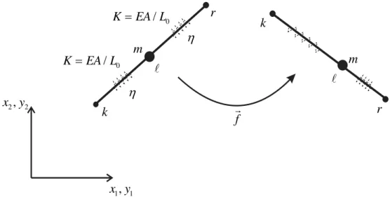
(21)2.3 Damping - Modified Kelvin/Voigt Model
the proposed model is called as Modified Kelvin Model. Before describing the proposed model it is important to note that, in general, it is not possible to find an explicit expression for the dissipative potential Q presented in equation (1), however, it is possible to write its internal force and,
there-fore, the variation of dissipation Q. A schematic representation of the proposed model can be seen
in Figure 2.
E E
,
E
S
S
Figure 2: Modified Kelvin/Voigt model adapted for Green strain.
From Figure 2 the Piola-Kirchhof stress is given by:
.
.
S
E
E
E
(22)for which the first term is the derivative of the specific strain energy in relation to the Green strain, see equation (11). So the second term corresponds to the dissipative part of the potential energy. For a finite element one writes the variation of the dissipative potential regarding nodal positions as:
0
0
0
0 0
0 0 0
.
.
fe
fe V
fe fe
i i
V
i i
fe
i i
V
i i
q
q
E
Q
Y dV
Y dV
Y
E Y
E
E
E
Y dV
E A L
Y
Y
Y
(23)where q is the dissipative potential by unit of volume (not written) and all variables are considered
constant for a truss element. Using equation (16) one defines the contribution of one element to the global dissipative force, as:
2 1
0 0 2
0
( 1)
.
fe fe
i vis i i
F
E A L
Y
Y
L
(24)
Considering all elements the variation of the dissipative potential results:
(vis)
i i
Q
F
Y
(25)To complete the consideration of viscosity, it should be mentioned that the solution proposed here is pure numerical and hence the speed of strain is calculated by the finite difference method in solution of nonlinear equilibrium equation. This strategy is originally described here for nonlinear strain measure, but was inspired in Mesquita and Coda (2002), Mesquita and Coda (2003) and Mesquita and Coda (2007) where linear viscoelastic models are proposed. As far as the authors knowledge goes it is different from all nonlinear viscoelastic formulations present in literature, see for example, Lemaitre and Chaboche (1990), Lemaitre (2001), Lima et al. (2015), Holzapfel (1996), Simo (1987), Huber and Tsakmakis (2000), Petiteau et al (2013), Marko et al. (2006) and Clough and Penzien (1985).
To introduce the numerical approximation one assumes a time step
t
and writes:t t t
E
E
E
t
(26)Substituting equation (26) into (24) results:
2 1
2 1
0 0 2 0 0 2
0 0
( 1)
( 1)
fe fe fe
i vis t t i i t t t i i t
F
E
A L
Y
Y
E A L
Y
Y
t
L
t
L
(27)Considering the time step sufficiently small one assumes:
2 1
2 1
i i t i i t t
Y
Y
Y
Y
(28)Comparing equations (27) and (17),one writes (27) as:
int
int
int
intfe fe fe fe
fe
i vis i t t i t i t t i t
F
F
F
F
F
t
t
E
(29)Therefore, the viscous internal force is numerically related to the elastic internal force.
3 NONLINEAR EQUILIBRIUM EQUATION AND SOLUTION PROCEDURE
Before introducing the Lagrange multipliers it is of interest to present the structure solution consid-ering the dissipative term concluding the description of main original contribution of this work. Substituting equations (4), (7), (18), (25) into equation (2) one writes:
(int) ( )
0
vis
i i i i i
F
M Y
F
F
Y
(30)As the position variation Yi
is arbitrary, equation (30) can be rewritten as:
(int) ( )
0
vis
i i i i i
F
F
M Y
F
(31)Or making the correspondence between the node number and the movement direction i
with a generic degree of freedom kd*
1
i (where d is the truss dimension 2D or 3D) one can(int) ( )
0
vis
F
F
M Y
F
(32) that is the nonlinear equation of dynamic equilibrium, or movement, of the analyzed structure.The adopted solution process combines: (i) the time integration of the dynamic equilibrium by the Newmark method, (ii) the original viscous force approximation by equation (29) and (iii) the Newton-Raphson nonlinear solver for equation (32).
Equation (32) is rewritten for a current instant (t t) as,
0
int int int
t t t t t t t t t t t t t
g
F
F
F
F
MY
CY
t
t
(33) or1
int int0
t t t t t t t t t t t
g
F
F
F
MY
CY
t
t
(34)where the mass proportional damping is also introduced, following Coda et al. (2013), Coda and Paccola (2014) and Coda and Paccola (2008), in order to not loss the generality. The Newmark approximations are used in the following form,
2
1
2
t t t t t t t
Y
Y
tY
t
Y
Y
(35)
1
t t t t t t
Y
Y
t
Y
tY
(36)where
t is a time step.Substituting equations (35) and (36) in equation (34) one finds:
1
20
int
t t t t t t t t
t t
int
t t t t t t
M
g Y
F
F
Y
Y
t
t
C
Y
MQ
CR
tCQ
F
t
t
(37)in which vectors Qt
, Rt
and int t
F represent the known dynamic contributions of the past. The in-ternal force int
t
F is calculated in the previous time step and stored to be used in the current instant,
values of Qt
and Rt
are given by:
2
1
1
2
t t t tY
Y
Q
Y
t
t
(38)
1
t t t
Equation (37) is nonlinear regarding
Ytt and can be summarized by g Y
tt 0. Itssolu-tion is done by the Newton-Raphson procedure from a Taylor expansion truncated at first order, as:
0
0
00
g( Y
tt)
g Y
tt
g Y
tt
Y
g Y
tt
Y
H
(40)where
2
02 2 2
1
1
t t
S
U
Q
M
C
M
C
g Y
Y
t
t
t
t
t
estat
H
H
(41)In equation (41) estat
H is the static hessian given, for each finite element, by equation (19). In
this equation the approximation described by equation (29) is employed, which implies that only the current viscous force depends on the current position and has influence in the dynamic hessian, see equation (37).
From equation (40) results the linear system of equation used to calculate a correction for the trial current position, i.e.,
0
0t t t t
g Y
Y
g Y
or
0t t
Y
g Y
H
(42)where 0
t t
Y is the trial position, usually adopted as Yt
at the begin of a time step. Solving Y a
new trial position Ytt
is calculated as
0
t t t t
Y
Y
Y
(43)This value of Ytt
is considered the new trial position 0 t t
Y
. The acceleration should be calcu-lated for each iteration by:
2
t t
t t t
Y
Y
Q
t
(44)Equation (44) is used to correct velocity in equation (36) and the iteration continues until,
0
g( Y )
TOL
or
Y /
X
TOL
(45)in which TOL is a pre defined tolerance. It is worth noting that Qt, Rt and int t
F are updated only at the end of the iterative procedure, i.e., at the beginning of the next time step. For the first time step the acceleration is calculated by:
1
0 0 0
0
U
Y
M
F
CY
Y
(46)4 INTRODUCTION OF THE LAGRANGE MULTIPLIER
Despite the damping described above can be used in any bar of the structure,in this section it is specially adapted to simulate the passive mass / spring / damper system of vibration control shown in Figure 3. This figure shows a mass / spring /damper system named z for which the stiffness is
2K, the damping parameter is 2 and the mass is m.
0
/
K
EA L
0
/
K
EA L
1
,
1x y
2
,
2x y
k
r
m
m
k
r
f
Figure 3: Vibration control device, 2D representation.
As the finite element simple bar (truss) cannot resist transverse loads it is necessary to con-strain the device mass movement to a straight line between nodes k and r of the system. The two equations to impose the necessary constraint for a three-dimensional device are:
2 2
1 1
2 2
1 1
0
r r k r k r
Y
Y
Y
Y
Y
Y
Y
Y
(47)and
3 3 3 3
1 1 1 1
r r k
k r k
Y
Y
Y
Y
Y
Y
Y
Y
or
3 3
1 1
3 3
1 1
0
r r k r k r
Y
Y
Y
Y
Y
Y
Y
Y
(48)The introduction of these constraints on the equilibrium equations is made by adding in the to-tal energy, equation (1), the sum of the following Lagrangian potentials
1 2 2 1 1 2 2 1 1
2 3 3 1 1 3 3 1 1
z r r k r k r
z
z z
z r r k r k r
L
L
Y
Y
Y
Y
Y
Y
Y
Y
Y
Y
Y
Y
Y
Y
Y
Y
(49)
where z varies from 1 to the number of installed devices nz, i.e.:
U
K
P
Q
L
The search of the stationarity is now made including the above restriction, as:
0
U
K
P
Q
L
(51)Remembering that the Lagrange multipliers are also free variables, it is written
ˆ
z z z
i z j i i j j
i j
L
L
L
Y
F
Y
Y
(52)where forces ˆ
i
F are actives when nodes belong to the devices z and
zj are the associated La-grange multipliers. Values of ˆi
F and z j
are given at appendix.
Using index notation over equation (51) and taking into account equation (52), equation (30) is rewritten as:
(int) ( )ˆ
0
vis z z
i i i i i i j j
F
M Y
F
F
F
Y
(53)This time, both Yi
and z j
are arbitrary, therefore,
ˆ
(int)
( )0
vis
i i i i i i
F
F
F
M Y
F
(54)and
0
s s
j j
(55)Equation (54) is very similar to equation (31), as the active coordinates of ˆ
i
F coincide with the coordinates of (int)
i
F . Equation (55) coincides with the imposed constraints, see equations (47) and
(48). Thus, the additional number of equations is
d1 *
nz where d is the dimension of thecon-sidered space (2D or 3D) and nz is the number of devices.
The solution process is identical to that described in the previous section where both the force vector (equations (A1) to (A11)) and the Hessian matrix will be changed. In the three-dimensional case, for a generic device z, one writes the terms to be added into the hessian matrix, as:
2 2
( )
2 2
( ) ( ) ( )
z z
z
i j i m
z
z z
z z z
n j n m
L
L
Y
Y
Y
L
L
Y
H
(56)
1 2 1 2 2 2 3 3
1 1 1 1
2 2 1 1
1 2 2 2 3 3
1 1 1
2 1 1
2 2 3 3
1 1
1 1
0
0
0
0
0
0
0
0
0
0
0
0
0
0
0
0
0
0
0
0
0
0
0
0
0
0
0
0
0
0
0
0
0
0
0
0
0
0
0
0
0
0
z z z z r r
z z r
z z r
z z r k r k
z k r
z k r
z
k k
k
k
Y
Y
Y
Y
Y
Y
Y
Y
Y
Y
Y
Y
Y
Y
Y
Y
Y
Y
Y
Y
SIM
Y
Y
Y
Y
H
(57)where the last two rows and columns correspond to the additional degrees of freedom per device. The other values are added to existent positions of the original hessian matrix. It is worth noting that in the solution process vectors Y and Y also contain the updating of Lagrange multipliers,
but these are not considered to calculate the acceptable error Y / X .
5 NUMERICAL SIMULATIONS
Some examples are shown to confirm the various aspects of the formulation. They are organized from very simple cases to more complicated ones.
5.1 Mass / Spring / Damper Device Validation
The example in figure 4 is solved statically, quasi-statically and dynamically. In static solution the contributions of mass and damping are neglected. An inclined force of F10 2kN is applied as
shown in figure 4. The physical properties of the bar are:
E
10GPa, 2 5A cm and L01m. From these values results a spring constant K5MN m/ , thus if Hooke's Law were used a horizontal
0
45
F
M 0/ 0
KE A L KE A0/L0
0
L L0
Figure 4: Lagrange multiplier validation.
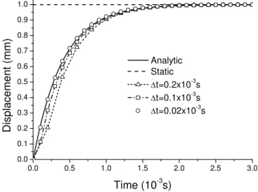
For this level of strain it is also expected that the quasi-static problem, including Kelvin/Voigt viscosity and discarding inertial forces, approaches the linear problem. Thus, the horizontal dis-placement as a function of time is given by /
0 0
( 2 / 2) (1 t ) / 2
h
u F L e E
E
A. One may thinkthis is the viscous damping equation however, for this simple problem, solutions are similar. Adopt-ing 4MPa s , figure 5 compares the achieved solutions for various time steps, revealing the
con-vergence of the proposed numerical viscoelastic approach to the analytical solution.
0.0 0.5 1.0 1.5 2.0 2.5 3.0
0.0 0.1 0.2 0.3 0.4 0.5 0.6 0.7 0.8 0.9 1.0
Di
spl
a
cem
e
n
t (m
m
)
Time (10-3s) Analytic Static
t=0.2x10⁻³s
t=0.1x10⁻³s
t=0.02x10⁻³s
Figure 5: Quasi-static results for the device.
In order to validate the damped dynamic model one employs bars density equal to
3 3
0 20 10x kg m/
. Thus, considering the others physical parameters one achieves the natural fre-quency of the device as
n1000rad s/ . Considering small strains the ratio between the maximum displacement amplitude u and the static displacement uh is given by1/ 2
2 2 2 2
/ h 1 / (1 / n) ( / )
u u E . Table 1 presents some results of / h
u u as a function of
/ n
for which is the excitation angular frequency. For the dynamic test one considers two force intensities F110 2kNcos(
t) and F21000 2kNcos(
t) as depicted in figure 4, with a time step of 410 t s
/ n
0.500 0.625 0.750 0.875 1.000 1.250 1.500 1.750 2.000
Anal. 1.288 1.518 1.885 2.374 2.500 1.329 0.721 0.459 0.322
Num.F1 1.289 1.521 1.893 2.394 2.531 1.334 0.722 0.459 0.322
Num.
2
F 1.281 1.505 1.858 2.336 2.526 1.349 0.723 0.460 0.323
Table 1:Maximum amplitude by the static displacement.
When the load is small the numerical response approaches better the linear response, for larger loads it was expected very different results, however, it is a good surprise that the damping behav-ior continues presenting the same pattern. For the purposes of this study the results are more than satisfactory, moreover the small difference indicates that it is possible to search better constitutive models to better fit the real device to be used.
5.2 Optimization of a Mass / Spring / Damper Device
In this and the next example it is used a hypothetical plane structure for representing a building with 12 floors, 36m in height and 5m in base. Its is used 49 truss finite elements with density
3 0 7000kg m/
, elastic modulus of E 210GPa and cross sectional area of 2
75.4 A cm .
The structure is constrained at the base by two fixed supports and the vibration control device is fixed at the top floor as indicated in figure 6. Figure 7 shows a detail of the device and the fixing strategy. The supporting bars have the same properties of other structural bars, but bars 1-2 and 2-3 of the device have elastic modulus E 1GPa, initial lenght
0 2.5
L m and cross sectional area 2
75.4 A cm .
Figure 7: Detail of the device.
The natural frequencies of the structure are calculated without and with the mass/spring device (not damped) by equation 1 2
0 0
M H I where H0 is the hessian matrix for the initial position that coincides with the linear stiffness matrix of the structure. The first frequency without the mass/spring device is 3.1253Hz when the device is coupled the first frequency is 0.963Hz.
Applying sinusoidal horizontal base movement in the same frequency of structures (with and without the mass/spring device) and with amplitude of 5cm, as both systems are not damped, the
resonance phenomenon takes place. The structure without the device reaches a top displacement amplitude of 6m in less than 5s, while the structure with the mass/spring (not damped) device reaches for the same period of time an amplitude less than 2 .m Thus, the introduction of the
mass/spring system without damping would have vibration control effect only for external actions of short duration.
Now it is introduced the modified Kelvin/Voigt damping
in the vibration control device as shown in equation (41). In order to optimize the device one varies from 410 s through 2 10 s
with a step of 3
10 s
. From previous analysis, it was found that with the damping variation there was a small variation in the natural frequency of the structure. Due to this reason it is neces-sary to vary the excitement frequencies from 0.963Hz through 1.04Hz with a step of 2
10
F Hz
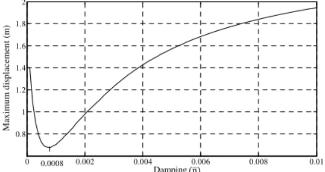
in order to find the worse excitation frequency for each damping parameter . Figure 8 shows the maximum displacement of the top of the structure as a function of the damping parameter for the worse possible excitation frequency. Figure 9 shows the worse frequency for each damping pa-rameter .
0 0.002 0.004 0.006 0.008 0.01 0.8
1 1.2 1.4 1.6 1.8 2
Damping
M
ax
imu
m d
isp
la
ce
me
n
t (m
)
0.0008
0 0.002 0.004 0.006 0.008 0.01 0.96
0.97 0.98 0.99 1 1.01 1.02 1.03 1.04
Damping
Fr
eque
nc
y
(
H
z)
0.0008 0.983
Figure 9: Frequency for which the maximum displacement occurs as a function of .
As detached in figure 8 the parameter
8 10x 4s minimizes the top displacement. In this case the frequency is approximately F0.983Hz. Figure 10 shows the displacement of the top of the structure as a function of time for these values of damping and frequency. As can be seen, in addi-tion to smaller amplitude, the presence of damping eliminates, as expected, the resonance profile. If a longer time is presented the maximum displacement stabilizes at 0, 7m as shown in figure 8.0 2 4 6 8 10 12 14 16
-0.8 -0.6 -0.4 -0.2 0 0.2 0.4 0.6 0.8
Time (s)
D
is
p
la
cem
en
t (
m
)
Figure 10: Top displacement as a function of time for the optimum damping.
The proposed device works very well and its use is not limited to small displacements as the formulation presents a geometrically exact description. One should note that the mass of the device developed horizontal and vertical movements keeping the alignment with nodes 1 and 3 of figure 7.
5.3 Structure under Earthquake-2D Model
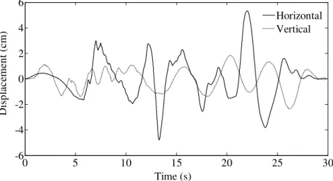
<http://peer.berkeley.edu/peer_ground_motion_database/spectras/21713/unscaled_searches/84357 /edit.>. The imposed base movements in horizontal and vertical directions are depicted in figure 11.
In addition to the mass / spring / damper device, the sliding base device is created by changing the configuration of the first floor, see Figure 12. As in the previous example 50 truss elements with density 3
0 7000kg m/
, elastic modulus
E
210GPa (with the exception of the diagonalelements) and cross sectional area of 4 75.4
A cm are adopted.
0 5 10 15 20 25 30
-6 -4 -2 0 2 4 6
Time (s)
D
ispl
ace
m
e
nt
(
c
m
)
Horizontal Vertical
Figure 11: Base movements in horizontal and vertical directions.
Figure 12: Sliding base device.
An optimization process is used to find the elastic modulus (
E
0.5GPa) of the cross diagonalsof the first floor limiting the base angle
to be less than 015 (see figure 12). The same damping
constant
8 10x 4s is adopted for diagonal bars of the first floor.floor and the horizontal acceleration of the top floor are evaluated. To perform this analysis four situations are considered: (i) without any vibration control device (ii) with vibration control mass / spring / damper (iii) with the sliding base device Figure 12 and (iv) with the combination of the two devices.
Figures 13 to 21 show results along time for the above described cases. As can be seen the slid-ing base device allows larger displacement amplitude, but reduces the frequency of the horizontal movement of the top floor. Regarding the acceleration of top floor, the device mass / spring / damper is the best. Regarding the behavior of the normal force on the right column of the second floor, both the sliding base device and the mass / spring / damper present equivalent performances.
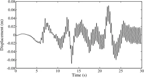
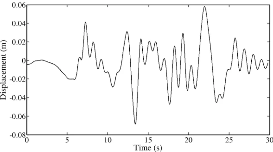
Now the combination of devices, case (iv), is analyzed and results are shown in figures 22, 23 and 24.
0 5 10 15 20 25 30
-0.08 -0.06 -0.04 -0.02 0 0.02 0.04 0.06 0.08
Time (s)
D
ispl
ace
m
ent
(
m
)
Figure 13: Displacement at the top floor - without devices.
0 5 10 15 20 25 30
-0.2 -0.15 -0.1 -0.05 0 0.05 0.1 0.15 0.2
Time (s)
D
ispl
ace
m
ent
(
m
)
0 5 10 15 20 25 30 -0.08
-0.06 -0.04 -0.02 0 0.02 0.04 0.06
Time (s)
Di
sp
la
ce
m
en
t (
m
)
Figure 15: Displacement of top floor - mass / spring / damper device.
0 5 10 15 20 25 30
-15 -10 -5 0 5 10 15
Time (s)
A
cc
ele
ta
tio
n
(m
/s
2 )
Figure 16: Acceleration at the top floor - without devices.
0 5 10 15 20 25 30
-20 -15 -10 -5 0 5 10 15 20
Time (s)
A
cc
ele
ta
tio
n
(m
/s
2 )
0 5 10 15 20 25 30 -2
-1.5 -1 -0.5 0 0.5 1 1.5
Time (s)
A
ccel
et
at
ion (
m
/s
2 )
Figure 18: Acceleration at the top floor - mass / spring / damper device.
0 5 10 15 20 25 30
-6 -5 -4 -3 -2 -1 0
Time (s)
N
o
rm
al
forc
e (
1
0
5 N)
Figure 19:Normal force without devices.
0 5 10 15 20 25 30
-3.6 -3.4 -3.2 -3 -2.8 -2.6 -2.4 -2.2 -2 -1.8
Time (s)
N
o
rm
al
forc
e
(10
5 N)
0 5 10 15 20 25 30 -7
-6 -5 -4 -3 -2
Time (s)
N
o
rma
l fo
rc
e
(1
0
5 N)
Figure 21: Normal force - mass / spring / damper device.
0 5 10 15 20 25 30
-0.2 -0.15 -0.1 -0.05 0 0.05 0.1 0.15
Time (s)
D
is
p
la
ce
me
n
t (m
)
Figure 22:Horizontal displacement at the top floor - sliding base and mass / spring / damper devices.
0 5 10 15 20 25 30
-0.8 -0.6 -0.4 -0.2 0 0.2 0.4 0.6
Time (s)
A
ccel
et
at
ion (
m
/s
2 )
0 5 10 15 20 25 30 -6
-5.5 -5 -4.5 -4 -3.5 -3 -2.5
Time (s)
N
o
rm
al
fo
rc
e
(10
5 N)
Figure 24:Normal force for sliding base and mass / spring / damper devices.
As shown in Figures 22, 23 and 24 the structure with two devices presents intermediate dis-placement in relation to the individual devices, moreover one can observe the beating profile. Fur-thermore, it was found that in this case the oscillations present larger periods. On the other hand, it should be noted that in terms of acceleration, this combination presents values lower than the mass-spring-damper system, thus offering more comfort to users. The device combination present an in-termediate maximum normal force amplitude. Thus, the combination of devices offers a better com-fort for users and improves the strength of the structure when compared to the sole mass / spring / damper device. Moreover, this example shows that the proposed viscoelastic rheological model is successfully implemented, is very stable and useful for general analysis.
5.4 3D Water Thank Tower
To confirm the possibilities and usefulness of the proposed formulation in practical analysis, in this example a 3D application is carried out with the intention of giving obvious and consistent results. The example consists of the analysis of a light structure that supports a water tank subjected to a horizontal impact with the composition of forces F11000kN and F2200kN with simultaneous duration of 0.1s. The force is applied as shown in Figure 25, causing overall effect of bending and
twisting. The plant structure is an equilateral triangle of side 2m. Vertical bars measuring 3m and diagonals, connecting the vertices of the larger triangle with the midpoints have length 10m. The connection device between the water tank and the structure (represented in red) is, at its initial position, parallel to y1 direction. Each bar of the device has ( 3 / 2)m in length. The thank connec-tion bars are present only at the top floor.
Displacements following y1, y2 and y3 directions of the loaded node are shown in figures 26 and 27 considering and not considering the modified Kelvin/Voigt damping for vertical (direction
3
M
1 2 3
1 F
2 F
1 y 2
y
Figure 25: Geometry and loading sketch.
All bars have the same cross section, circular tubes with radius R6cm and thickness 0.05
t cm. Structural bars, i.e., without damping, have
7000kg m/ 3 andE =
210GPa. For thethank connection bars it is adopted
E
0.2GPa,
2000kg m/ 3 and0.1s
. When base vertical bars are considered damped, the adopted viscous parameter is 1.0s. The water tank mass is
considered M 16000kg and its dead weight P160kN.
0 10 20 30 40 50 60 70
-0,8 -0,6 -0,4 -0,2 0 0,2 0,4 0,6 0,8 1
Time (s)
Di
sp
la
ce
m
e
n
t (m
)
y
1 direction
y
2 direction
y
3 direction
0 10 20 30 40 50 60 70 -0.6
-0.4 -0.2 0 0.2 0.4 0.6 0.8
Time (s)
D
is
p
lacem
en
t (
m
)
y
1 direction
y
2 direction
y
3 direction
Figure 27: - Displacement of the loaded node with base damping.
Due to the Lagrange multiplier technique, the water tank is constrained to move along the straight line between nodes 1 and 3. Figure 28 shows some selected positions of the tower move-ment.
The proposed examples reveal that the mass / spring / damping device is working properly for 2D and 3D applications. Example 1 shows that the rheological model and the Lagrange Multiplier technique are appropriate to static and dynamic application and unify approaches. Examples 2, 3 and 4 show that the formulation is able to model large displacement situations using large strain mass / spring / damping devices. Furthermore, the success of numerically integrating the Kelvin-Voigt rheological model opens the possibility of developing more realistic models for nonlinear dy-namic damping.
6 CONCLUSIONS
This study presents a total Lagrangian formulation to perform nonlinear dynamic analysis of plane and space trusses. For this total Lagrangian formulation it is proposed an original Lagrangian mul-tiplier and a modified Kelvin viscoelastic constitutive model approach to consider sliding mass / spring / damper devices for vibration control. The more important contribution is the proposed modified Kelvin viscoelastic constitutive model that make possible assembling damping for static and dynamic analysis from phenomenological viscosity at large strain using the Green strain meas-ure. The main advantage of this formulation, when compared to the classical ones, is the possibility of its extension to comprise more complex viscous behavior without the necessity of analytically solving differential equations. An interesting surprise of technical interest is the same damping be-havior of the modified Kelvin model for small and large displacements and strains. The success of numerically integrating the Kelvin-Voigt rheological model opens the possibility of developing more realistic models for nonlinear dynamic damping and its extension to 3D viscoplastic analysis.
Acknowledgements
Authors thank FAPESP (São Paulo Research Foundation) for the financial support of this research.
References
Armero, F. (2006). Energy-dissipative momentum-conserving time-stepping algorithms for finite strain multiplicative plasticity, Computer Methods in Applied Mechanics and Engineering, 195 (37-40): 4862-4889.
Bathe, K.J., Ramm, E., Wilson, E.L., (1975). Finite element formulations for large deformation dynamic analysis. Internat. J. Numer. Methods Engrg., 9, 353–386.
Bauchau, O.A., Bottasso, C.L. (2001). Contact Conditions for Cylindrical, Prismatic, and Screw Joints in Flexible Multibody Systems. Multibody System Dynamics, 5 (3): 251-278.
Bonet, J., Wood, R.D., Mahaney, J., Heywood, P. (2000). Finite element analysis of air supported membrane struc-tures, Computer Methods in Applied Mechanics and Engineering, 190: 579-595.
Clough, R.W.,. Penzien, J. (1975). Dynamics of structures, MacGraw-Hill.
Coda, H.B., Paccola, R.R. (2008). A positional FEM Formulation for geometrical nonlinear analysis of shells. Latin American Journal of Solids and Structures, 5 (3), 205-223.
Coda, H.B., Paccola, R.R. (2014). A total-Lagrangian position-based FEM applied to physical and geometrical non-linear dynamics of plane frames including semi-rigid connections and progressive collapse. Finite Elem. Anal. Des., 91: 1-15.