Abstract
This paper proposed an integrated algorithm of neuro-fuzzy tech-niques to examine the complex impact of socio-technical influenc-ing factors on road fatalities. The proposed algorithm could handle complexity, non-linearity and fuzziness in the modeling environ-ment due to its mechanism. The Neuro-fuzzy algorithm for deter-mination of the potential influencing factors on road fatalities consisted of two phases. In the first phase, intelligent techniques are compared for their improved accuracy in predicting fatality rate with respect to some socio-technical influencing factors. Then in the second phase, sensitivity analysis is performed to calculate the pure effect on fatality rate of the potential influencing factors. The applicability and usefulness of the proposed algorithm is illus-trated using the data in Iran provincial road transportation sys-tems in the time period 2012-2014. Results show that road design improvement, number of trips, and number of passengers are the most influencing factors on provincial road fatality rate.
Keywords
Road Fatalities, socio-technical factors, road transportation sys-tems, Neuro-fuzzy.
Determination of the Main Influencing Factors on Road
Fatalities Using an Integrated Neuro-Fuzzy Algorithm
1 INTRODUCTION
Road fatalities can be subject to many influencing factors that may from one country or region to another. Road fatality may be influenced by socio-technical-economical factors, cultural factors, road design factors, vehicle mix on road, etc. Although significant correlation may be reported be-tween the changes in fatalities and the influencing factors, the type of functional characteristics remains undetermined to practitioners and policy makers. There is a need to develop reliable and robust methods to examine the effect of influencing factors on fatality rate.
Road safety performance has been the subject of many research works. Tingvall et al. (2010) studied the relationship between middle output indicators and final safety indicators and using a regression model they showed the significance of relationship between middle output indicators such
Amir Masoud Rahimi a
a Assistant Professor, Civil Engineering
Department, Faculty of Engineering, University of Zanjan, Zanjan, Iran. Email: [email protected]
http://dx.doi.org/10.1590/1679-78253106
as behavior modification and technology utilization, and fatality rate. Ma et al (2011) categorized road safety indicators according to the geographical areas including regional, urban, and highway. Kulmala (2010) emphasized the need for a comprehensive framework in which different safety as-pects including exposure rate, accident risk, and unwanted outcome management had been taken into consideration.
In the aggregate data context, factors that serve as surrogates for exposure to traffic crashes are generally classified as socioeconomic and demographic features (e.g., GNP, or amount of income tax, per capita alcohol consumption, literacy rate, total/urban population and vehicle densities, em-ployment rate, the distribution of population by age class, by matrimonial status, number of suicide and of drug offences, number of hospitals and medical personnel, etc.), road network characteristics including environmental and engineering features (e.g., mean precipitation, mean number of rain, frost, hail, fog, and snow days, curvatures, presence of ramps, number of lanes, etc.), policymaking (e.g., road classification/ construction), driver behavior (e.g., age chords and rate of driver licens-ing), vehicle characteristics, and police enforcements (e.g., speed limit regulation and seat-belt legis-lation) in a county/city/country (Anwaar et al., 2012; Coruh et al., 2015; Jamroz, 2015).
Gitelman et al. (2013) focused on safety indicators in managing post-accident unwanted conse-quences. They introduced five groups of safety indicators including emergency service accessibility, emergency personnel accessibility, emergency facilities accessibility, response time to emergency calls, and hospital bed accessibility for accident injuries. Yannis et al. (2013) studied behavioral indicators (safety belt utilization, to avoid alcohol and drug usage) along with vehicle indicators (vehicle reliability, air bag) and discussed the need for other safety indicators including policy, infra-structure, management and intelligent technologies (see also Christoph et al. (2013) for more vehicle related indicators).
Rohayu et al. (2012) used a time-series (ARIMA) to model changes in fatality rate in Malaysia and predicted road fatalities for the year 2020. Macinko et al., (2015) studied the effect on motor vehicle fatalities of the two influencing factors position in the car and the sex of the driver. Burke and Nishitateno (2015) studied the effect of gasoline price on road fatalities and showed that a 10% increase in the gasoline pump price will result in 3%–6% decline in fatalities. Castillo-Manzano et al. (2015) examined the impact on the traffic accident rate of the interaction between trucks and cars on Europe’s roads using a panel data in 1999–2010. They reported that increasing the relative num-ber of trucks lead to higher traffic fatalities. Ahangari et al. (2015) studied the improvement trends in road fatalities in 16 industrialized countries on a basis of structural factors, gasoline price, socio-economic factors, mobility levels, motorization, and health care.
AI techniques are increasingly diversifying today but between them two techniques have gained special attention in function estimation problems namely Artificial Neural Networks (ANN) and adaptive neuro-fuzzy inference system (ANFIS) (Jang et al., 1997). Due to the ability of neural networks and neuro-fuzzy system in modeling complex nonlinear systems, plenty of their successful applications have been reported in the literature in different fields.
This paper is organized as follows. In section 2, a step-by-step neural networks and neuro-fuzzy system algorithm is presented. Section 2 also introduces the theory of the methods. Section 3, pre-sents the results of the proposed algorithm for modelling the relationship between influencing factors and fatalities in 31 provinces of Iran. Section 4 presents the main findings and conclusion.
2 NEURO-FUZZY ALGORITHM
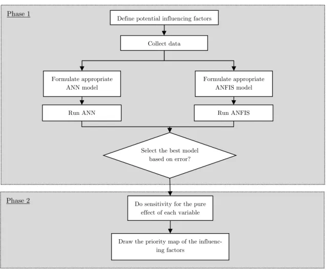
The neuro-fuzzy algorithm for determination of the potential influencing factors on road fatalities is depicted in Figure 1. This algorithm consists of two phases. In the phase 1, first, all the potential influencing factors with significant effect on fatality rate are specified based on a survey in the re-lated literature. Then, data on the specified variables are collected. In the next two parallel steps, ANN and ANFIS models are formulated and then got trained with the train data. At the end of phase 1, ANN and ANFIS are compared regarding their error for test data (capability for predic-tion) and the best method is selected based on minimum error. Therefore, the main output of the first phase is the best method for modelling and estimation of fatality rate.
In the second phase, sensitivity analysis is performed to calculate the pure effect on fatality rate of the potential influencing factors. It should be noted that this sensitivity analysis is performed with the use of the preferred best method from phase 1. Finally, a priority map of the influencing factors will be drawn and those factors with the relative high impact on fatality rate will be deter-mined.
2.1 Data on the Influencing Factors
For study the fatality rate and its changes over years in different provinces, some influencing factors are derived and the data are collected. These influencing factors are:
Daily transit: the number of vehicles passed a special point in the road, discovered by traffic moni-toring cameras
Number of road improving projects in a province, eliminating dangerous points
Number of intelligent technologies (ITS) installed along all road in the province
Number of emergency stations along all road in the province
Number of users trained for better road safety
The share of highway in the total length of provincial roads
The share of illuminated roads in the total length of provincial roads
The total number of trips in a year in a province
The total number of passengers delivered in every 100 KM
Population density; the number of people in every 100 KM of roads
Fatalities; number of users died on the provincial roads
Figure 1: The Neuro-fuzzy algorithm to determine the influencing factors on fatalities.
Model Variables Min Max Average STDEV
Daily transit, 6552 218208 43786 46524
Road design improvement 3 76 19 15
ITS in 100 KM 1 18 6 4
Emergency service 16 107 41 25
User training 2874 27984 9183 5799
Highway share in 100 KM 2 65 22 14
Road illumination in 100KM 1 30 7 7
Population 459754 11860666 2447182 2198878
# of trips (thousands) 84 1478 570 364
# of passengers 1463 26533 6741 5830
Fatalities 10 1023 356 210
Road network size (length) 375 7877 2722 1820
Source: RMTO, 2015
Table 1: Descriptive Statistics of the Model Variables. Phase 2
Phase 1
Define potential influencing factors
Draw the priority map of the influenc-ing factors
Formulate appropriate ANFIS model
Run ANFIS Collect data
Do sensitivity for the pure effect of each variable Formulate appropriate
ANN model
Run ANN
2.2 Artificial Neural Network
The research in the field has a history of many decades, but after a diminishing interest in the 1970's, a massive growth started in the early 1980's. Today, Neural Networks can be configured in various arrangements to perform a range of tasks including pattern recognition, data mining, classi-fication, forecasting and process modeling. ANNs are composed of attributes that lead to perfect solutions in applications where we need to learn a linear or nonlinear mapping. Some of these at-tributes are: learning ability, generalization, parallel processing and error endurance. These attrib-utes would cause the ANNs solve complex problem methods precisely and flexibly.
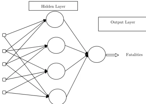
ANNs consists of an inter-connection of a number of neurons. There are many varieties of con-nections under study, however here we will discuss only one type of network which is called the Multi Layer Perceptron (MLP). In this network the data flows forward to the output continuously without any feedback. Figure 2 shows a typical two-layer feed forward model used for road fatality forecasting.
Figure 2: A two-layer MLP network.
The input nodes are the previous lagged observations while the output provides the forecast for the future value. Hidden nodes with appropriate nonlinear transfer functions are used to process the information received by the input nodes. The model can be written as:
0 0
1 1
n m
t j ij t i j t
j i
y f y (1)
Where m is the number of input nodes, n is the number of hidden nodes, f is a sigmoid transfer function such as the logistic:
Influencing factors
Hidden Layer
Output Layer
1 ( )
1 exp( )
f x
x
{ j, j = 0, 1, ..., n} is a vector of weights from the hidden to output nodes and { ij, i = 1, 2, …, m; j = 0, 1, …, n}are weights from the input to hidden nodes. 0 and oj are weights of arcs leading from the bias terms which have values always equal to 1. Note that Equation (1) indicates a linear transfer function is employed in the output node as desired for forecasting problems.
The MLP’s most popular learning rule is the error back propagation algorithm. Back Propaga-tion learning is a kind of supervised learning introduced by Werbos (1974).At the beginning of the learning stage all weights in the network are initialized to small random values. The algorithm uses a learning set, which consists of input – desired output pattern pairs. Each input – output pair is obtained by the offline processing of historical data. These pairs are used to adjust the weights in the network to minimize the Sum Squared Error (SSE) which measures the difference between the real and the desired values over, all output neurons and all learning patterns. After computing SSE, the back propagation step computes the corrections to be applied to the weights.
The attraction of MLP has been explained by the ability of the network to learn complex rela-tionships between input and output patterns, which would be difficult to model with conventional algorithmic methods. There are three steps in solving an ANN problem which are 1) training, 2) generalization and 3) implementation. Training is a process that network learns to recognize present pattern from input data set. We present the network with training examples, which consist of a pattern of activities for the input units together with the desired pattern of activities for the output units.
For this reason each ANN uses a set of training rules that define training method. Generaliza-tion or testing evaluates network ability in order to extract a feasible soluGeneraliza-tion when the inputs are unknown to network and are not trained to network. We determine how closely the actual output of the network matches the desired output in new situations. In the learning process the values of interconnection weights are adjusted so that the network produces a better approximation of the desired output. ANNs learn by example. They cannot be programmed to perform a specific task.
The examples must be selected carefully otherwise useful time is wasted or even worse the net-work might be functioning incorrectly. The disadvantage is that because the netnet-work finds out how to solve the problem by itself and its operation can be unpredictable. In this paper the effort is made to identify the best fitted network for the desired model according to the characteristics of the problem and ANN features.
2.3 Adaptive Network-Based Fuzzy Inference System (ANFIS)
the fusion of fuzzy and neural network technologies as it facilitates an accurate initialization of the network in terms of the parameters of the fuzzy reasoning system.
A specific approach in neuro-fuzzy development is the adaptive neuro-fuzzy inference system (ANFIS), which has shown significant results in modeling nonlinear functions Jang et al. (1997). ANFIS uses a feed forward network to search for fuzzy decision rules that perform well on a given task. Using a given input-output data set, ANFIS creates a FIS whose membership function param-eters are adjusted using a backpropagation algorithm alone or a combination of a backpropagation algorithm with a least squares method. This allows the fuzzy systems to learn from the data being modeled. For more details the interested readers are referred to Jang et al. (1997).
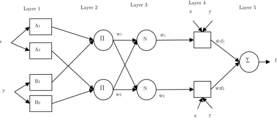
Adaptive Neuro-Fuzzy Inference Systems are fuzzy Sugeno models put in the framework of adaptive systems to facilitate learning and adaptation. Such framework makes FLC more systemat-ic and less relying on expert knowledge. To present the ANFIS architecture, let us consider two-fuzzy rules based on a first order Sugeno model:
Rule 1: if (x is A1) and (y is B1) then (f1 = p1x + q1y + r1)
Rule 2: if (x is A2) and (y is B2) then (f2 = p2x + q2y + r2) (2)
One possible ANFIS architecture to implement these two rules is shown in Figure 3. In the fol-lowing presentation OLi denotes the output of node i in a layer L.
Figure 3: Construct of ANFIS
Layer 1: All the nodes in this layer are adaptive nodes, i is the degree of the membership of the input to the fuzzy membership function (MF) represented by the node:
2
1, 1,
( ) ( )
i
i
i A
i B
o x
o y (3)
Ai and Bi can be any appropriate fuzzy sets in parameter form.
ŵ2f2
ŵ1f1
ŵ2
ŵ1
w1
w2
A1
∏ ∏
N N
∑
A2
B1
B2
x
y
x y
f x y
Layer 2: The nodes in this layer are fixed (not adaptive).These are labeled M to indicate that they play the role of a simple multiplier. The outputs of these nodes are given by:
2,i i Ai( ) Bi( ),
o w x y i=1, 2 (4)
The output of each node is this layer represents the firing strength of the rule.
Layer 3: Nodes in this layer are also fixed nodes. These are labeled N to indicate that these per-form a normalization of the firing strength from previous layer. The output of each node in this layer is given by:
3,
1 2
i i
i i
i
w w
o w
w w
w (5)
Layer 4: All the nodes in this layer are adaptive nodes. The output of each node is simply the product of the normalized firing strength and a first order polynomial:
4,i i i i( i i i)
o w f w p x q y r i=1, 2 (6)
Where pi, qi and ri are design parameters (consequent parameter since they deal with the then-part of the fuzzy rule).
Layer 5: This layer has only one node labeled S to indicate that is performs the function of a simple summer. The output of this single node is given by:
5,
i i i
i i i
i i
i w f
o w f
w (7)
The ANFIS architecture is not unique. Some layers can be combined and still produce the same output. In this ANFIS architecture, there are two adaptive layers (1, 4). Layer 1 has three modifia-ble parameters (ai, bi and ci) pertaining to the input MFs. These parameters are called premise parameters. Layer 4 has also three modifiable parameters (pi, qi and ri) pertaining to the first order polynomial. These parameters are called consequent parameters (Jang et al., 1997).
3 RESULTS
The data on the influencing factors as well as the fatality rate are collected for the 31 provinces in Iran in the time period 2012-2014. Therefore, totally 93 data observations are available to train and test the methods. For training, 80% of the data available are used to run ANN and ANFIS. To have robust and accurate results and to eliminate the effect of variable scales, all data are normal-ized between 50 and 100.
algo-rithm is the error back-propagation named trainlm. The transfer function for the hidden layer is Sigmoid function and for output layer is Linear.
For ANFIS training, the input variables should be represented in terms of fuzzy linguistic vari-ables. Here, we use subtractive clustering algorithm. First, genfis2 function of MATLAB® has gen-erated an initial FIS and then this initial FIS is trained by anfis function to yield a final fuzzy in-ference system named ANFIS.
After training, ANN and ANFIS are compared for their better performance according to their forecasting error. The error estimation method used in this study is Mean Absolute Percentage Er-ror (MAPE). It can be calculated by the following equation:
1
1 n t
t t
x x
MAPE
n x (8)
In (8), x and xare actual and estimated data, respectively. Scaling the output, MAPE method is the most suitable method to estimate the relative error because input data may have different scales.
Figure 4 illustrates the performance of ANN and ANFIS for modeling and estimation of fatality rate. As seen, the estimated fatality rate by ANN is closer to the actual data than the estimated fatality rate by ANFIS. In this figure, the MAPE for ANN is 4.3% and for ANFIS is 6.3%, both error rates are satisfactory but the error of ANN is lower than ANFIS.
0 2 4 6 8 10 12 14 16 18
50 55 60 65 70 75
province-year
no
rm
aliz
ed
fa
ta
lit
y
ra
te
ANN Actual ANFIS
Figure 4: Comparison of ANN and ANFIS for fatality rate prediction.
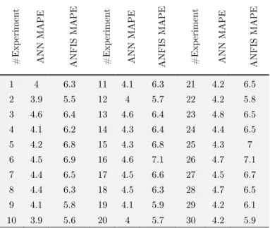
The results of MAPE in the above Table 1 show that the error of ANN with the average of 4.3% is significantly less than the error of ANFIS with the average of 6.3%. Therefore, with respect to MAPE, the preferred method for modelling fatality rate is ANN.
#Experiment AN
N M
A
PE
ANFIS M
A
PE
#Experiment AN
N M
A
PE
ANFIS M
A
PE
#Experiment AN
N M
A
PE
ANFIS M
A
PE
1 4 6.3 11 4.1 6.3 21 4.2 6.5 2 3.9 5.5 12 4 5.7 22 4.2 5.8 3 4.6 6.4 13 4.6 6.4 23 4.8 6.5 4 4.1 6.2 14 4.3 6.4 24 4.4 6.5 5 4.2 6.8 15 4.3 6.8 25 4.3 7 6 4.5 6.9 16 4.6 7.1 26 4.7 7.1 7 4.4 6.5 17 4.5 6.6 27 4.5 6.7 8 4.4 6.3 18 4.5 6.3 28 4.7 6.5 9 4.1 5.8 19 4.1 5.9 29 4.2 6.1 10 3.9 5.6 20 4 5.7 30 4.2 5.9
Table 2: The results of MAPE in the randomly conducted experiments.
3.1 Impact Analysis With ANN
Figure 5 shows the pure effect of daily transit on road fatality rate. As seen this effect is very small that cannot be significant however, the small changes are non-linear.
50 55 60 65 70 75 80 85 90 95 100
64.4 64.6 64.8 65 65.2 65.4 65.6 65.8 66
Daily transit
no
rm
aliz
ed
fa
ta
lity
ra
te
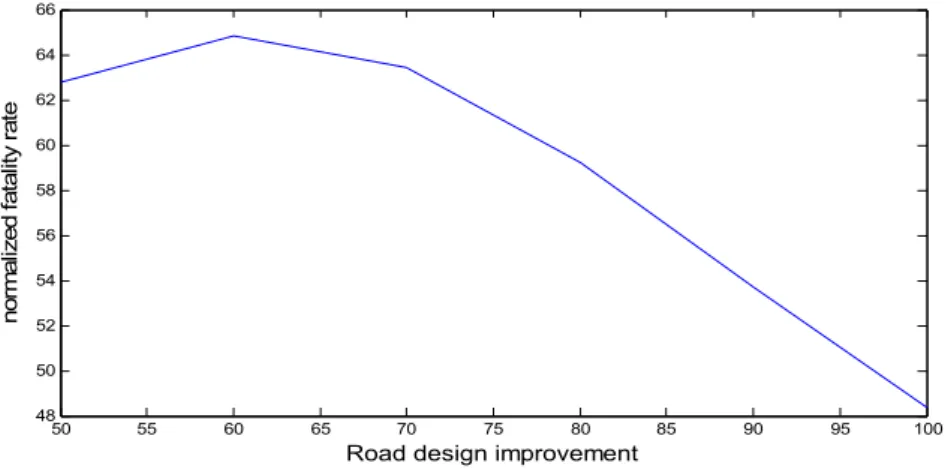
Figure 6 shows the pure effect of road design improvement on road fatality rate. As seen this ef-fect is significant and the changes are non-linear.
Figure 7 shows the pure effect of intelligent technologies on road fatality rate. As seen this ef-fect is not significant yet the changes are non-linear.
50 55 60 65 70 75 80 85 90 95 100
48 50 52 54 56 58 60 62 64 66
Road design improvement
no
rm
al
iz
ed
fa
ta
lity
ra
te
Figure 6: The pure effect of road design improvement on provincial road fatalities.
50 55 60 65 70 75 80 85 90 95 100
63 63.5 64 64.5 65 65.5
ITS in 100 KM
no
rm
al
iz
ed
fat
al
ity
ra
te
Figure 7: The pure effect of intelligent technologies on provincial road fatalities.
50 55 60 65 70 75 80 85 90 95 100 65 66 67 68 69 70 71 72 73 Emergency service no rm ali ze d fa ta lit y ra te
Figure 8: The pure effect of emergency services on provincial road fatalities.
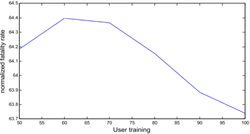
50 55 60 65 70 75 80 85 90 95 100 63.7 63.8 63.9 64 64.1 64.2 64.3 64.4 64.5 User training no rm al iz ed fa tal ity rat e
Figure 9: The pure effect of user training on provincial road fatalities.
Figure 10 shows the pure effect of highway share on road fatality rate. As seen this effect is sig-nificant and the changes are non-linear. Figure 11 shows the pure effect of road illumination on road fatality rate. As seen this effect is significant and the changes are non-linear.
50 55 60 65 70 75 80 85 90 95 100 58 60 62 64 66 68 70 72 74
Highway share in 100 KM
nor mal iz ed fa ta lit y ra te
50 55 60 65 70 75 80 85 90 95 100 63 64 65 66 67 68 69 70 71 72
Road illumination in 100KM
no rm aliz ed fa ta lit y ra te
Figure 11: The pure effect of road illumination on provincial road fatalities.
Figure 12 shows the pure effect of number of trips services on road fatality rate. As seen this ef-fect is significant and the changes are linear. Figure 13 shows the pure efef-fect of number of passen-gers on road fatality rate. As seen this effect is significant and the changes are linear. Figure 14 shows the pure effect of population density on road fatality rate. As seen this effect is significant and the changes are non-linear.
50 55 60 65 70 75 80 85 90 95 100
55 60 65 70 75 80 85 90 95 100 105
# of trips
nor m al iz ed fat al ity rat e
Figure 12: The pure effect of number of trips on provincial road fatalities.
50 55 60 65 70 75 80 85 90 95 100 48 50 52 54 56 58 60 62 64 66 68
# of passengers
no rm aliz ed fa ta lity ra te
In summary, the effects of the influencing factors normalized between -1 to +1 are presented in Figure 15. Assuming all these effects are distributed according to a Normal distribution, the lower and upper bound in this figure shows a distance of one standard deviation from the mean, i.e. [μ-σ, μ+σ]. Those pure effects which lay outside of this confidence interval are considered as the most influencing factors on road fatality rate. As seen in this figure, the influencing factors 1, 8, and 9 are the most influencing factors which are road design improvement, number of trips, and number of passengers.
50 55 60 65 70 75 80 85 90 95 100
60 65 70 75 80 85
population density
no
rm
al
iz
ed
fa
tal
ity
rat
e
Figure 14: The pure effect of population density on provincial road fatalities.
Figure 15: The normalized pure effect of influencing on provincial road fatalities.
4 CONCLUSIONS
intel-ligent techniques namely ANN and ANFIS to find the complex impact of socio-technical influencing factors on road fatalities. The proposed algorithm could handle complexity, non-linearity and fuzzi-ness in the modeling environment. The neuro-fuzzy algorithm for determination of the potential influencing factors on road fatalities consisted of two phases. In the first phase, ANN and ANFIS were compared regarding their accuracy for fatality prediction and ANN was determined as the preferred method. In the second phase, ANN based sensitivity analysis was performed to calculate the pure effect on fatality rate of the potential influencing factors. Results showed that road design improvement, number of trips, and number of passengers are the most influencing factors on road fatality rate.
References
Ahangari, H., Atkinson-Palombo, C., & Garrick, N. W. (2015). Assessing the Determinants of Changes in Traffic Fatalities in Developed Countries. Transportation Research Record: Journal of the Transportation Research Board, 1(2513): 63-71. DOI: http://dx.doi.org/10.3141/2513-08
Anwaar, A., Anastasopoulos, P., Ong, G.P., Labi, S., Bin Islam, M., (2012). Factors affecting highway safety, health care services, and motorization – an exploratory empirical analysis using aggregate data. Journal of Transportation Safety and Security 4 (2): 94–115. DOI: 10.1080/19439962.2011.619372
Brown, M., Harris, C., (1994). Neurofuzzy Adaptive Modeling and Control, Prentice Hall, New Jersey, USA. Burke, P. J., & Nishitateno, S. (2015). Gasoline Prices and Road Fatalities: International Evidence. Economic In-quiry, 53(3): 1437-1450. DOI: 10.1111/ecin.12171.
Castillo-Manzano, J. I., Castro-Nuño, M., & Fageda, X. (2015). Can cars and trucks coexist peacefully on highways? Analyzing the effectiveness of road safety policies in Europe. Accident Analysis & Prevention, 77: 120-126. doi:10.1016/j.aap.2015.01.010
Christoph M., Martijn Alexander Vis, Lucy Rackliff, Henk Stipdonk, A road safety performance indicator for vehicle fleet compatibility, Accident Analysis & Prevention, 60(2013): 396-401, doi:10.1016/j.aap.2013.07.018
Coruh, E., Bilgic, A., & Tortum, A. (2015). Accident analysis with aggregated data: The random parameters nega-tive binomial panel count data model. Analytic Methods in Accident Research, 7: 37-49.
Gitelman, V., Auerbach, K., & Doveh, E. (2013).Development of road safety performance indicators for trauma management in Europe. Accident Analysis & Prevention, 60: 412-423. Doi:10.1016/j.aap.2012.08.006
Jamroz, K. (2015). Country Safety Performance Function and the factors affecting it. Signals and Systems: A Primer with MATLAB®, 101.
Jang, J.S.R., (1993). ANFIS: adaptive network based fuzzy inference system. IEEE Transactions on Systems Man Cybernetics, 23(3): 665–683. DOI: 10.1109/21.256541
Jang, R., Sun, C., Mizutani, E. (1997). Neuro-fuzzy and soft computation, Prentice Hall, New Jersey.
Kulmala R (2010). Ex-ante assessment of the safety effects of intelligent transport systems, Accident Analysis & Prevention, 42(4):1359-1369. doi:10.1016/j.aap.2010.03.001.
Ma, Z., Shao, C., Ma, S., & Ye, Z. (2011). Constructing road safety performance indicators using fuzzy delphi meth-od and grey delphi methmeth-od. Expert Systems with Applications, 38(3): 1509-1514. doi:10.1016/j.eswa.2010.07.062. Macinko, J., Silver, D., &Bae, J. Y. (2015). Age, period, and cohort effects in motor vehicle mortality in the United States, 1980–2010: The role of sex, alcohol involvement, and position in vehicle. Journal of safety research, 52: 47-57 Doi:10.1016/j.jsr.2014.12.003.
Rohayu, S., Sharifah Allyana, S. M., Jamilah, M. M., & Wong, S. V. (2012). Predicting Malaysian road fatalities for year 2020.
Tingvall, C., Stigson, H., Eriksson, L., Johansson, R., Krafft, M., & Lie, A. (2010). The properties of Safety Perfor-mance Indicators in target setting, projections and safety design of the road transport system. Accident Analysis & Prevention, 42(2): 372-376.Doi: 10.1016/j.aap.2009.08.015.
Werbos, P.I. (1974). Beyond Regression: New Tools for Prediction and Analysis in the Behavior Sciences. Ph.D. Thesis, Harvard University, Cambridge, MA.