Lat. Am. j. solids struct. vol.13 número5

(1)

Abstract

In this work, the influence of uniaxial and biaxial partial edge loads on buckling and vibration characteristics of stiffened lami-nated plates is examined by using finite element method. As the initial pre-buckling stress distributions within an element are highly non-uniform in nature for a given loading and edge condi-tions, the critical loads are evaluated by dynamic approach. To-wards this, a nine-node heterosis plate element and a compatible three-node beam element are developed by employing the effect of shear deformation for both the plate and the stiffeners respective-ly. In the structural modeling, the plate and the stiffener elements are treated separately, and then the displacement compatibility is maintained between them by using a transformation matrix. Ef-fect of different parameters such as loaded edge width, position of loads, boundary conditions, ply-orientations and stiffener factors are considered in this study. Buckling results show that the uniaxi-al loaded stiffened plate with around (+30o/-30o)2 layup can

with-stand higher load irrespective of boundary conditions and loading patterns, whereas the maximum load resisting layup for the bi-axially loaded stiffened plate is purely dependent on edge conditions and loading patterns.

Keywords

Stiffened laminates, partial edge load, buckling, vibration, finite element method, heterosis element

Effects of Partial Edge Loading and Fibre Configuration

on Vibration and Buckling Characteristics

of Stiffened Composite Plates

T. Rajanna a,* Sauvik Banerjee b Yogesh M. Desai c D. L. Prabhakara d

a_{Research Scholar,}b_{Associate Professor,}

c_{Professor, Department of Civil}

Engi-neering Indian Institute of Technology Bombay, Mumbai-400 076, India

d_{Director, Sahyadri College of}

Engineer-ing and Management, Mangalore-575 007, India

*_{Assistant Professor, Department of}

Civil Engineering, B.M.S. College of Engineering (Autonomous College under VTU), Bengaluru-560 019, India

E-mails: a [email protected]

b_{[email protected]}

c_{[email protected]} d_{[email protected]}

http://dx.doi.org/10.1590/1679-78252239

(2)

1 INTRODUCTION

Composite laminates belong to a category of thin-walled structures that are commonly being used in many applications like aerospace, civil, marine, and mechanical engineering structures. These laminates have been extensively used in weight sensitive aircrafts and aerospace industries since their inception, and recently in civil engineering structures such as bridge decks, bridge girders, strengthening and retrofitting of existing structures.

Higher strength/weight ratio, high specific stiffness, enhanced fatigue life are some of the well-known characteristics of composite materials. These characteristics are further enhanced by adding stiffener to a plate without considerably affecting its overall weight. For a negligible weight penalty, there is an enormous increase in the strength and stability characteristics throughout the structures. Plates with an array of stiffeners are commonly found in fuselage and wings of an aircraft, a ship’s hull and its deck, offshore drilling rigs, pressure vessels, roofing units, launching pedestal of rocket, etc. The diverse applications of such stiffened plates are found to be exposed to in-plane edge loading in many situations. The presence of these loadings may significantly alter the free vi-bration response of such stiffened plates. In fact, a situation may arise wherein the natural frequen-cy of a component becomes zero, thereby causing instability of the component at a fairly low-stress field. Hence, the problem of elastic stability may be considered as a special case of vibration prob-lems, and such problems are of considerable importance and interest to researchers for many years.

Many past studies have reported on stability and/or vibration characteristics of stiff-ened/unstiffened plates with uniform compressive edge loads (Kamruzzaman et al., 2006; Khedmati and Edalat, 2010; Mirzaei et al., 2015; Sayyad and Ghugal, 2014; Sayyad et al., 2016; Singh and Chakrabarti, 2012). However, such uniform edge compressions are unusual in practice. Many practi-cal situations demand the stiffened plate subjected to concentrated and partial edge loads.

(3)

under uni-/bidirectional partial edge loading conditions using FE method was investigated by Sundaresan et al. (1998). The same problem was further explored by Sahu et al. (2001) with an extension to the vibration behaviour of laminated plates under different edge loads. Srivastava et al. (2003) examined the critical buckling behaviour of isotropic stiffened plates with partial and con-trated loads using FE approach. The free vibration characteristics of isotropic stiffened plates are studied by Hamedani et al. (2012) using super finite element technique. The same problem and techniques were further extended to get buckling results by Hamedani and Ranji (2013).

It has been observed that, in finite element formulation, most of the authors have used eight-node serendipity elements by considering the effect of shear deformation. Some authors (Palani et al., 1989; Palani et al., 1992; Pugh et al., 1978) have noticed that for certain mesh configuration boundary conditions, the eight-node plate element locks in shear, even when selective or reduced integration techniques are used for a thin plate configuration. It is also stated that the eight-node serendipity element is comparatively more sensitive to element aspect ratios and element shape distortions (Palani et al., 1989) whereas, the nine-node Lagrange element exactly interpolates the quadratic displacement fields and has nearly optimal performance (Palani et al., 1989; Pugh et al., 1978). However, some of the authors (Butalia et al., 1990; Hughes and Cohen, 1978) have also found that the nine-node Lagrange element locks in shear, even when reduced or selective integra-tion techniques are employed for thin plates. In fact, the stiffness matrix exhibits rank deficiency resulting in the appearance of spurious mechanisms, i.e. zero energy modes (Butalia et al., 1990; Hinton and Owen, 1984; Hughes and Cohen, 1978). These communicable mechanisms may result in erratic solution. These shortcomings, namely locking and spurious mechanisms, have led to the de-velopment of a heterosis element by employing serendipity shape functions for transverse degree of

freedom w, and Lagrange shape functions for rotations θx and θy (Butalia et al., 1990; Hughes and

Cohen, 1978). This element exhibits improved characteristics as compared to each of the previous quadratic elements and offers high accuracy for extremely thin plate configuration (Hughes and Cohen, 1978). The same element has been used in this study by considering the effect of in-plane

displacements u, v in addition to transverse and rotational displacements.

From this brief overview of the past literature, it is observed that a large body of research work has been carried out on the buckling characteristics of plates under uniform edge compression. On the contrary, relatively less amount of research works deal with the partial in-plane edge compres-sion. Further, the buckling behaviour of isotropic stiffened plates under partial in-plane edge com-pression is sparsely treated in the literature. To the best knowledge of the authors, no comprehen-sive work is identified in the literature regarding in-plane partial edge load for stiffened laminated plates. The present work deals with the problem of vibration and buckling of stiffened composite laminates under the action of in-plane partial edge loads.

(4)

2 FORMULATION OF EQUATIONS WITH THEORY

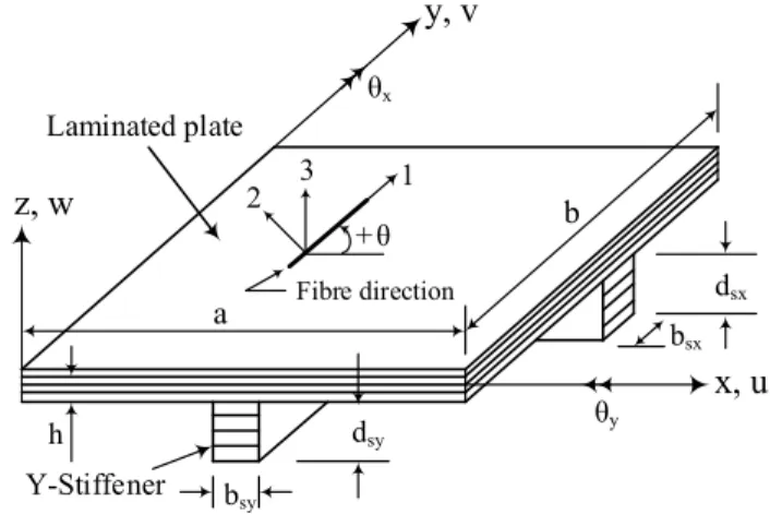
The geometrical configuration of the bidirectional stiffened laminated plate of plan-form (a x b)

with stiffeners parallel to x and y directions is shown in Figure 1. The middle-plane displacement

fields corresponding to x, y, and z directions are u, v, and w, respectively.

Laminated plate

Fibre direction 1

+θ 3 2

y, v

a

b z, w

x, u θy

θx

bsx dsx

dsy h

Y-Stiffener _b_sy

Figure 1: Laminate geometry of the plate with bidirectional stiffeners.

2.1 Strain-Displacement Relations

Lagrange’s strain displacement equations are used throughout the formulation. The expressions pertaining to the linear strain relation of the plate by considering the effect of shear deformation are given by

x

xy

y

xyl

x xz

yz

xl

yl u

z x v

z y

u v

z

y x

w x w y

c c

c

q q

g

g g

e

üïï

+ _ïï

ïï ïï

+ _ïï

ïï ïï ïï

+ _ýï

ïï ïï ï

+ _ïï

ïï ïï ï +

ïïïþ ¶

¶ ¶ ¶

¶ _{¶ +}

¶ ¶

¶ ¶ ¶ ¶ =

=

(1)

where xl, yl and xyl are the linear in-plane normal and shear strains; xz and yz are transverse shear

strains; z is the distance of any layer from the middle plane of the plate and χ are the curvatures.

(5)

2 2

2 2 2

2

2 2 2

2

1 1 1 1

2 2 2 2

1 1 1 1

2 2 2 2

y x

u v w

z

x x x x x

u v w

z

y y y y y

xnl ynl q q q q

e

ù

æ¶ ö

éæ ö

æ¶ ö_÷ æ¶ ö_÷ æ¶ _÷ö _ç¶ _÷ _ç _÷ _ú

ç ç ç ê ÷

= çèç¶ ø÷÷ + èçç¶ ÷ø÷ + èçç¶ ÷÷ø + ëçêçè¶ ø÷÷ + çççè¶ ÷÷ø úú_û

é ¶

æ¶ ö_÷ æ¶ ö_÷ æ¶ ö_÷ æ¶ ö_÷

ç ç ç çê

= ç_ç_¶ ÷ +_÷_÷ ç_ç_¶ _÷_÷÷ + ç_ç_¶ _÷÷ +_÷ _ê_çç_¶ _÷_÷÷ + _¶

è ø è ø è ø _ëè ø

2

2 x x y y

u u v v w w

z

x y x y x y x y x y

xynl q q q q

g

üïï ïï ïï ïï ï ù ï

æ ö_÷ _ú _ï_ï

ç _÷

ç ÷ ú ý

ç ÷

ç ï

è ø ú_û _ï

ïï ï ù

¶ ¶

æ ö é ï

æ ö ¶ ¶

¶ ¶ ¶ ¶ _ç¶ _÷_ç_{¶ ÷} _ê _ú_ï

= ¶ ¶ +¶ ¶ +èçç¶ ÷ç÷øèç¶ ø÷÷÷ + ëê¶ ¶ + ¶ ¶ ú_ûïïþïïï

(2)

where in, θx and θy are the rotations of normal to the un-deformed mid-plane of the plate about y

and x axes, respectively.

The stress-strain relation for a lamina with reference to the plate axes is given by

{ } _ij

{ }

_l

k

Q

s _{= ê ú}é_ë ù_û e ₍₃₎

By using Equations (1) and (3), the constitutive relation for the laminated plate can be given by

{

}

{

}

{ }

0 0 0 0

p p p

p

ij ij j

i

p p p p

i ij ij j

p _p _p

i ij j

A B

N

M B D

Q S

e c g

é ù ì ü

ì ü é ù é ù ï ï

ï ï _ê_ê _ú _ê _ú _ú_ï _ï

ï ï ë û ë û ï ï

ï ï _ê _{ú ï} _ï

ï ï _ï _ï

ï ï₌ êé ù é ù úï ï

í ý _ê_ê_ë _{ú ê}_{û ë} _ú_û _úí ý

ï ï ï ï

ï ï ê úï ï

ï ï _ê _é _ù_úï ï

ï ï ï ï

ï ï ê ê úúï ï

î þ ë ë û ïû î ïþ

in short form,

{

_NP

}

é_DPù

{ }

_eP

= êë úû (4)

where

 

T

P P P P

i x y xy

N  N N N _ are stress resultants,

 

P P P P T

i x y xy

M  M M M _ are moment resultants,

 

_P _P _P T

i xz yz

Q  Q Q _ are transverse shear stress resultants; likewise,

 

P P P P T

j x y xy

 _{ }   _ are the middle

plane strains,

 

P P P P T

j x y xy

 _{ }   _ _{are the middle plane curvatures and}

 

T

P P P

j xz yz

 _{ }  _ _{are the}

trans-verse shear strains. From Eq. (4), the extension-extension P

ij

A

 

 , extension-bending   BijP and

bend-ing-bending P

ij

D

 

  of the stiffness components can be expressed as

(

)

( )

(

)

-1

2

1

, , k 1, z, , , 1, 2, 6 k

n z P P P

ij ij ij ij _k z k

A B D Q z dz i j

=

å ò

= ₍₅₎

and

( )

-1 1

, , 4, 5 k

k

n z

P

ij ij _k

z k

S a Q d z i j

=

å ò

= ₍₆₎

in which n is the number of layers, is the shear correction factor, which is given by 5/6 (Kolli and

Chandrashekhara, 1996; Reddy, 1996) and   Qij _kis the stiffness matrix of k

th_{lamina with reference}

to plate axes (Reddy, 1996).

(6)

{

sx

}

sx

{ }

sx

N = ëéD ù_û e ₍₇₎

{

sy

}

sy

{ }

sy

N = ëéD ù_û e ₍₈₎

where

 

_sx _sx _sx _sx _sx T

x x xy xz

N  N M M Q _ and

 

sx sx sx sx sx T

x x xy xz

 _{ }    _ are the stress resultants and middle

plane strains for the stiffener, respectively; sx

D

 

 is the modified reduced constitutive matrix, which

is obtained by ignoring the resultant stresses



sx sx sx sx 0



y xy y yz

N N M Q  but not strains



sx sx sx sx 0



y xy y yz

     in the Eq. (4) and upon simplification, the reduced constitutive matrix of

x-stiffener is obtained (Kolli and Chandrashekhara, 1996). A similar procedure is adopted to obtain

the reduced constitutive matrix, sy

D

 

  of y-stiffener.

2.2 Finite Element Formulation

In the present work, the plate has been discretized using nine-node (9-N) heterosis plate element

with five degrees of freedom (DOF) given as u, v, w, θx and θy at all edge nodes and four DOF such

as u, v, θx and θy at the inside node. The serendipity shape functions have been used for transverse

DOF w, and Lagrange shape functions for remaining DOF that includes u, v, θx, θy as shown in

Figure 2. In a discretization of stiffener, three-node beam element with four DOF at each node has

been used viz., u, w, θx, θy for x-stiffener and v, w, θx, θy for y-stiffener. However, the other two

kinds of quadratic elements such as eight-node (8-N) serendipity and nine-node (9-N) Lagrange elements have also been considered in this study as illustrated in Figure 2. The results of these quadratic elements are given only in comparison studies along with the results of heterosis element.

8-N Serendipity 9-N Heterosis 9-N Lagrange

Node with u, v, w, θx, θy degrees of freedom Node with u, v, θx, θy degrees of freedom

Figure 2: Different types of plate elements.

2.2.1 Elastic Stiffness Matrices

The total strain energy due to linear strains in the entire stiffened plate is given by

{ } { }

1 1 1

2 2 2

L _T L L

T T

p p sx sx sy sy

L l _j j l j j l j j

j v j v j v

U e s dv e s dv e s dv

= = =

=

å

_ò

+

å

_ò

+

å

_ò

₍₉₎

where L is the number of elements of the plate or the x-stiffener or the y-stiffener involved in the

(7)

 

l 

 

B d

 

e ,in terms of derivatives of nodal shape functions and its corresponding displacement

vectors, the linear part of the total strain energy can be obtained as,

{ }

1 1 , 2 L

T p sx sy

L e e

j

U d k k k d

=

éé ù é ù é ùù

=

å

_ê_ë_{ë û}+_ë _û+_ë _û_ú_û

{ } { }

1

,

2

T p sx sy

d ééK ù éK ù éK ùù d

= _ê_ë_ë _û+_ë _û+_ë _û_ú_û

{ } [ ]{ } 1

,

2

T

d K d

=

(10)

where

 

de and

 

d are the elemental and global displacement vectors, respectively;

P

k ,

 

  _ksx_ and

sy

k

 

  are the element elastic stiffness matrices for plate, x-stiffener and y-stiffener, respectively;  _{ }K

is the global stiffness matrix of the entire stiffened plate and are expressed as,

1 1

-1 -1

,

T

p p p p

p

k B D B J d dx h

+ +

é ù = é ù é ù é ù

ë û

ò ò

ë û ë û ë û (11)

-1

,

T T

sx sx sx sx sx sx sx

k E B D B E J dx

+

é ù = é ù é ù é ù é ù é ù

ë û

ò

ë û ë û ë û ë û ë û (12)

-1

,

T T

sy sy sy sy sy sy sy

k E B D B E J dh

+

é ù = é ù é ù é ù é ù é ù

ë û

ò

ë û ë û ë û ë û ë û (13)

where sx

E

 

 and_Esy_are the transformation matrices;  _{ }BP ,_Bsx_and_Bsy_are the elemental strain

displacement matrices for plate, x-stiffener and y-stiffener, respectively, wherein

9

9 9

9

1,2..8

0 0 0 0 0 0 0

0 0 0 0 0

0 0 0 0 0 0 0

0 0 0

i i i i i P i i i i i i i i N N x x N N y y

N N N N

y x y x

N N x x B N N y N N y x N N x N N y ₌

é¶ ù ¶

ê ú

ê ¶ ú ¶

ê _¶ ú _¶

ê ú

¶ ¶

ê ú

ê_¶ _¶ ú _¶ _¶

ê ú

ê _¶ _¶ ú _¶ _¶

ê ú

ê _¶ ú _¶

ê ú

ê _¶ ú _¶

é ù₌ ê ú

ê ú ê ú

ë û _ê ¶ _ú ¶

ê _¶ ú

ê ú

¶ ¶

ê ú

ê ¶ ¶ ú

ê _¶ ú

ê ú

ê _¶ ú

ê ú

ê _¶ ú

ê ú

ê _¶ ú

ë û 9 9 9 9 9 0 0

0 0 0

y

N N

y x

N

é _é _ùù

ê _ê _úú

ê _ê _¶ _úú

ê _ê _úú

ê _ê _¶ _¶ _úú

ê _ê _úú

ê _ê _¶ _¶ _úú

ê _ê _úú

ê _ë _ûú

ë û

(8)

and

1,3

0 0 0

;

0 0 0 0 0 0

0 0 0 0

sy sx _i i sy sx i i sx sy i i sx _sy sx

i i sy

i _i sx sy i N N y x N N y x N N x y

N _N N

N

x _y

B B

=

é¶ ù

é¶ ù ê ú

ê ú _ê _¶ _ú

ê ¶ ú ê ú

ê ú _ê _¶ _ú

ê ¶ ú _ê _ú

ê ú _ê _¶ _ú

ê ¶ ú _ê _ú

é ù ₌ _ê _ú é ù ₌ _ê _ú

ë û _ê _¶ _ú ë û _¶

ê ú

ê ú _ê _ú

ê ¶ ú _ê ¶ _ú

ê _¶ ú _ê _ú

ê ú _ê ¶ _ú

ê ú _ê _ú

ê ¶ ú

ë û ê_ë ¶ ú_û

(15)

and also

3 3

1 1

1 0 0 0 0 1 0 0

0 0 1 0 0 0 0 1 0 0

;

0 0 0 1 0 0 0 0 1 0

0 0 0 0 1 0 0 0 0 1

sx sy i i sx sy e e E E = =

é ù é ù

ê ú ê ú

é ù = ê ú é ù = ê ú

ë û _ê _ú ë û _ê _ú

ê ú ê ú

ë û ë û

å

(16)

in which esx 



dsxh / 2



and esy 



dsyh / 2



are stiffener eccentricities.

2.2.2 Geometric Stiffness Matrices

The total strain energy due to non-linear strains in the entire stiffened plate is given by

{ } { }

1 1 1

2 2 2

L _T L L

T T

p p sx sx sy sy

L l _j l _j _j l _j _j

j

j _v j _v j v

U e s dv e s dv e s dv

= = =

=

å

_ò

+

å

_ò

+

å

_ò

₍₁₇₎

Substituting the non-linear strain displacement of plate [Eq. (2)] and the corresponding stiffen-ers in the above equation and upon simplification, we get the final form of Eq. (17) as given below:

{ }

1 1 , 2 NL L

T p sx sy

e G G G e

j

U d k k k d

=

å

_ê_ë_{ë û}+_ë _û+_ë _û_ú_û

{ } { }

1

,

2

T p sx sy G

G G

d ééK ù éK ù éK ùù d

= _ê_ë_ë _û+_ë _û+_ë _û_ú_û

{ }

[

]

{ } 1 , 2 T G

d K d

= (18) where P G k ,  

  kGsxand sy G

k

 

 are the elemental geometric stiffness matrices for plate, x-stiffener and

y-stiffener, respectively; KG is the overall geometric stiffness matrix of the entire stiffened plate,

which are expressed as,

1 1

-1 -1

,

G G G

p p T

p p

p

k B S B J d dx h

+ +

é ù= é ù é ù é ù

ë û

ò ò

ë û ë û ë û (19)

-1

,

G G G

T T

sx sx sx sx sx sx sx

k E B S B E J dx

+

é ù₌ é ù é ù é ù é ù é ù

(9)

[ ]

[

]

[

]

[ ]

[

]

[

]

-1

,

G G G

T T

sy sy sy sy sy sy

sy

k E B S B E J dh

+

=

_ò

₍₂₁₎

where P

G

B ,

 

  BGsxand sy G

B

 

 are the elemental non-linear strain displacement matrices for plate,

x-stiffener and y-x-stiffener, respectively; P

S ,

 

  _Ssx_and sy

S

 

 are the corresponding initial pre-buckling

stress matrices, in which

9

1,2..8

0 0 0 0 0 0 0

0 0 0 0

i i i i i i i i i i i P G N N x x N N y y N x N y N x N y N x N y N x N y B =

é¶ ù ¶

ê ú

ê¶ ú ¶

ê_¶ ú _¶

ê ú

ê_¶ ú _¶

ê ú

ê _¶ ú

ê ú

ê _¶ ú

ê ú

ê _¶ ú

ê ú

ê _¶ ú

ê ú

ê ¶ ú

ê ú

ê _¶ ú

é ù₌ _ê _ú

ê ú

ë û ê ¶ ú

ê ú

ê ¶ ú

ê _¶ ú

ê ú

ê _¶ ú

ê ú

ê _¶ ú

ê ú

ê _¶ ú

ê ú

ê _¶ ú

ê ú

ê _¶ ú

ê ú

ê ¶ ú

ê ú

ê ¶ ú

ë û 9 9 9 9 9 9

0 0 0

0 0 0 0

0 0 0

N x N y N x N y N x N y

é _é _ùù

ê _ê _úú

ê _ê ¶ _úú

ê _ê _úú

ê _ê ¶ _úú

ê _ê _¶ _úú

ê _ê _úú

ê _ê _¶ _úú

ê _ê _úú

ê ê ¶ úú

ê _ê _úú

ê ê ¶ úú

ê _ê _¶ _úú

ê _ê _úú

ê _ê _ú

ê _ê ¶ _ú

ê _ê _¶ _ú

ê _ê _ú

ê _ê _¶ _ú

ê _ê _ú

ê _ê _¶ _ú

ê _ê _ú

ê _ê _¶ _ú

ë û êë û ú ú ú ú ú ú ú ú ú ú (22) and 1,3

0 0 0

sx i sx i sx G sx i sx i i N x N x N x N x B =

é¶ ù

ê ú

ê ¶ ú

ê ú

ê ¶ ú

ê ú

ê ¶ ú

é _{ù = ê} _ú

ë û _ê _¶ _ú

ê ú

ê ¶ ú

ê _¶ ú

ê ú

ê ¶ ú

ë û (23) and 1 1 2 2

[ ] 0 0 0

0 [ ] 0 0

0 0 [ ] 0

0 0 0 [ ]

sx sx sx sx sx s s s s S é ù ê ú ê ú ê ú ê ú

é ù =

ë û _ê _ú

ê ú

ë û

(10)

in which

0 0

1

[Ssx] = d_sxs sx = N sx (25)

3 2

0 0

2 12 12

[_Ssx] ₌ dsx _s sx ₌ dsx _N sx ₍₂₆₎

2.2.3 Consistent Mass Matrices

The abbreviated form of total kinetic energy in the entire stiffened plate by including the effect of in-plane inertia, transverse inertia and rotational inertia is as follows:

{ }

1

, 2

L _T

p sx sy

e e

j

T d m m m d

=

å

 _ê_ë_ë _û+_ë _û+_ë _û_ú_û 

{ }

1

, 2

T _p _sx _sy

d ééM ù éM ù éM ùù d

=  _ê_ë_ë _û+_ë _û+_ë _û_ú_û 

{ }

[ ]

{ }

1

, 2

T

d M d

=  

(27)

where as P

m ,

 

  _msx_and sy

m

 

 are the elemental mass matrices for plate, x-stiffener and y-stiffener,

respectively;  _{ }M is the overall mass matrix of the entire stiffened plate, which are expressed as,

1 1

-1 -1

,

T p p p

p

m N I N J d dx h

+ +

é ù é ù é ù

é _{ù =} _ê _{ú ê ú ê} _ú

ë û

ò ò

ë û ë û ë û (28)

-1

,

T sx T

sx sx sx sx sx sx

m E N I N E J dx

+

é ù é ù é ù

é ù₌ é ù _ê _{ú ê} _{ú ê} _úé ù

ë û

ò

ë û ë û ë û ë ûë û (29)

-1

,

T sy T

s y sy sy sy sy sy

m E N I N E J dh

+

é ù é ù é ù

é ù= é ù _ê _{ú ê} _{ú ê} _úé ù

ë û

ò

ë û ë û ë û ë ûë û (30)

in which

1 2

1

2 3

0 0 0

0 0 0 0

0 0 0

p

I I

I

I I

I

é ù

ê ú

é _{ù = ê} _ú

ê ú

ë û ê ú

ê ú

ë û

(11)

and

1 2

1

2 3

3

0 0

0 0 0

0 0

0 0 0

sx

I I

I

I I

é ù

ê ú

é _{ù = ê} _ú

ê ú

ë û _ê _ú

ê ú

ë û

(32)

with

(

)

(

)

-1

2

1

1 , 2 , 3 1 , , z .

k

z L

k k _z

z dz

I

r

=

å ò

₍₃₃₎

2.3 Governing Equations

The governing equation of motion for vibration and stability problems derived using extended Ham-ilton’s principle is given below:

(

)

{ }

2

1

0 .

t

T U dt

D

_ò

- = ₍₃₄₎

where T is the kinetic energy for entire stiffened plate, U is the strain energy due to linear and

non-linear strains; t1, t2 are two arbitrary values of time t and Δ denotes the variational operator.

Substituting Eqns (10), (18) and (27) into the Eq. (34) and upon simplification, the following most general governing differential equation of motion is obtained as follows:

[ ]{ }

M q



+

[ ]

K

{ }

q

-

P K

[ ]

_G

{ }

q

=

0 .

{ }

₍₃₅₎

The governing equations for the vibration and buckling can be obtained separately by reducing Eq. (35) as follows:

Vibration problem: When the stiffened/unstiffened plate vibrates harmonically with a given in-plane load, Eq. (35) reduces to

[ ]

_-

[

]

{ } _- 2[ ]{ } { }_{0 .}

G

K P K q w M q

é ù ₌

ë û (36)

Buckling problem: when

   

q  0 ,Eq. (35) reduces to

[ ]

K

{ }

q

-

P K

_cr

[ ]

_G

{ }

q

=

0 ,

{ }

₍₃₇₎

where Pcr is the critical load and P is the applied edge compression.

Both Eqs (36) and (37) represent the eigenvalue problems. The square of frequency, ω2_{, for an}

applied in-plane load P is the eigenvalue in Eq. (36) and the critical load Pcr is the eigenvalue in

Eq. (37).

(12)

3 NUMERICAL RESULTS AND DISCUSSIONS

3.1 Computer Program

The solution of stability problems using either dynamic or static approach involves extraction of eigenvalues and eigenvectors, as evidenced in Eqs (36) and (37) respectively. The large sized matri-ces appearing in these two equations have to be stored in skyline form. Bathe (1996) has given the time-tested code in FORTRAN for extraction of the eigenvalues using the subspace iteration tech-nique. To be compatible with this, the FORTRAN code has been developed to generate various element level and global matrices and finally stored these matrices in skyline assembled form.

In the code, a selective integration scheme is incorporated for the generation of element elastic stiffness matrix. A 3 x 3 Gauss rule is adopted for membrane as well as bending effects while 2 x 2 Gauss rule is adopted for shear effects. As the geometric stiffness matrix is a function of the buckling stress field in an element due to the application of any kind of in-plane loads, it is a pre-requisite to perform the plane stress analysis before the generation of geometric stiffness matrix. Hence, code is done for the plane stress analysis to evaluate the stress field at 3 x 3 Gauss points. Accordingly, the integration for the generation of geometric stiffness matrix has been done using 3 x 3 Gauss rule (full integration). Similarly, A 3 x 3 Gauss rule is adopted to evaluate element level mass matrix also.

3.2 Boundary Conditions, Stiffener Parameters and Material Constants

In the present work, for the configuration of the stiffened laminated plate shown in Figure 1, two types of boundary conditions have been employed are as follows:

(1) Simply supported (S-S-S-S):

(i) for initial pre-buckled stress analysis: along the edges (a) x = 0, a; w = θy = 0, (b) y

= 0, b; w = θx = 0 and at x = a/2, u = 0; at y = b/2, v = 0

(ii) for buckling analysis: along the edges (a) x = 0, a; u = w = θy = 0, (b) y = 0, b; v

= w= θx=0.

(2) Clamped supported (C-C-C-C):

(iii) for initial pre-buckled stress analysis: along the edges (a) x = 0, a; w = θx = θy = 0,

(b) y = 0, b; w = θx = θy = 0 and at x = a/2, u = 0; at y = b/2, v = 0

(i) for buckling analysis: along the edges (a) x = 0, a; u = v = w = θx = θy = 0, (b) y

= 0, b; u = v = w = θx = θy= 0.

The stiffener dimensions are decided according to the non-dimensional parameters, in which

and are defined as: = nAs/bh which is the ratio of total area of the stiffeners to that of the

plate, where n is the number of stiffeners and As is the cross-sectional area of each stiffener;

similar-ly, = nE2Is /bD is the ratio of total bending stiffness of the stiffeners to that of the plate, where Is

is the moment of inertia of the stiffener about the plate centroidal axis and D is the flexural rigidity

of the plate, which is _D_ _Eh3_{/12(1 -}_2₎_{for isotropic case and} 3 2

2 /12(1 - 12)

D  E h  for composite case.

The ratio of thickness of plate to the width of the plate (h/b) is considered as 0.01 unless otherwise

(13)

The vibration frequency and the critical loads are represented in non-dimensional form as given in Table 1 and the elastic material properties with reference to the principal axes have been given in Table 2 unless otherwise mentioned.

Parameters Stiffened/unstiffened plates

Isotropic Composite

Natural frequencies(ϖ) b2 h D/ b2 h E h/ ₂ 2 Buckling load (cr) Pcrb2/D Pcrb2/E2h3

Table 1: Non-dimensional parameters (Deolasi et al., 1995; Leissa and Ayoub, 1988; Reddy and Phan, 1985).

In Table 1, ω is the absolute value of frequency, ρ is the material density, D is the flexural

ri-gidity of the plate and Pcr is the absolute critical buckling load.

Material Stiffened/unstiffened plates

E11 E22 G12 G13 G23 ν12

Isotropic 1.0 1.0 0.3854 0.3854 0.3854 0.30

Composite 25.0 1.0 0.50 0.50 0.20 0.25

Table 2: Material constants (Reddy, 1996; Sundaresan et al., 1998; Xiao et al., 2008).

3.3 Comparative Studies

The validation of the finite element formulation described above is necessary to ascertain the cor-rectness of the development of various matrices involved in the analysis of vibration and buckling problems. From the comparative studies of deflections and rotations for unstiffened/stiffened plates subjected to lateral loads, one can ascertain the validity of the elastic stiffness matrix. After ascer-taining this, if the vibration frequencies are compared, the formulation of the mass matrix can be validated. Finally, if the buckling loads are compared with the classical/numerical solutions, the generation of the geometric stiffness matrix can be validated. Validation of all these matrices has been carried out as described in the following sub-sections.

3.3.1 Static Analysis of Laminated Stiffened and Unstiffened Plates

The values of deflection of unstiffened/stiffened laminated plates under lateral loads are determined and the results are represented in Table 3 and Table 4, respectively. The effect of uniformly

distrib-uted load ( )q on the central deflection( )W of a laminated plate is tabulated in Table 3 along with

the results of Reddy (1996) and 3D-FEM solutions (Xiao et al., 2008). The results show very good agreement with the analytical solution. Table 4 shows the central deflection of a laminated square plate with centrally placed bidirectional stiffeners subjected to various boundary conditions with the

material properties pertaining to AS4/3501 graphite/epoxy composite: E11 = 144.8 GPa; E22 = 9.65

(14)

geomet-rical dimensions of the stiffened plate [see Figure 1] are as follows: a = 254 mm, b = 254 mm, h =

12.7 mm, bsx = bsy = 6.35 mm and dsx = dsy = 25.4 mm. The results using nine-node heterosis

ele-ment and eight-node serendipity eleele-ment are depicted in Table 4. It can be observed that both the elements give satisfactory results. However, the results of heterosis element seem to be more accu-rate when compared to those obtained from eight-node element and nine-node element, which was previously used by Kolli and Chandrashekhara (1996). The satisfactory agreement of the results with the literature clearly shows the correctness in the formulation of element elastic stiffness

ma-trix for both plate P

k

 

  as well as stiffeners_ksx_ and sy

k

   .

Source b/h 0 0/90/0 0/90/90/0 0/90/0/90/0 ((0/90/90)0)₂

Closed-form (Reddy, 1996)

10

0.952 1.022 1.025 0.973 0.964

3D-FEM(Xiao et al., 2008) 0.948 1.154 1.140 1.058 --

Present (heterosis) 0.952 1.022 1.025 0.973 0.957

20

0.726 0.757 0.769 0.758 0.758

3D-FEM(Xiao et al., 2008) 0.726 0.795 0.803 0.779 --

100 0.653 0.670 0.683 0.687 0.690

Table 3: Non-dimensionalised central deflection 3 4

max 2

w w E h / qa 2

( )10 for different cross-ply

laminated simply supported unstiffened square plate.

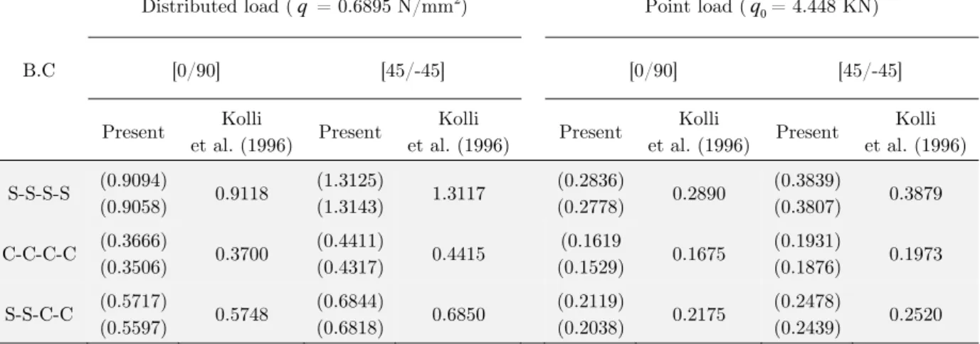
B.C

Distributed load (q = 0.6895 N/mm2) Point load (q₀= 4.448 KN)

[0/90] [45/-45] [0/90] [45/-45]

Present Kolli

et al. (1996) Present

Kolli

Kolli et al. (1996)

S-S-S-S (0.9094)

(0.9058) 0.9118

(1.3125)

(1.3143) 1.3117

(0.2836)

(0.2778) 0.2890

(0.3839)

(0.3807) 0.3879

C-C-C-C (0.3666)

(0.3506) 0.3700

(0.4411)

(0.4317) 0.4415

(0.1619 )

(0.1529) 0.1675

(0.1931)

(0.1876) 0.1973

S-S-C-C (0.5717)

(0.5597) 0.5748

(0.6844)

(0.6818) 0.6850

(0.2119)

(0.2038) 0.2175

(0.2478)

(0.2439) 0.2520

Note: Values within the first parentheses indicate the result from nine-node heterosis element and those in second parentheses from eight-node serendipity element.

(15)

3.3.2 Vibration Study of Laminated Unstiffened and Stiffened Plates

To further validate the formulation of the mass matrix, the free vibration characteristics of an un-stiffened square composite plate are studied using nine-node heterosis element (9-NHE); the results are presented in Table 5 along with the closed-form solutions (CFS) given by Reddy and Phan (1985). However, to ascertain the performance of other kinds of elements, the authors have also studied the free vibration behaviour using nine-node Lagrange element (9-NLE) and eight-node serendipity element (8-NSE). It is concluded that the adoption of nine node heterosis element in the formulation is a better choice than the use of other elements.

Table 5: Non-dimensionalised frequency of an angle-ply laminated simply supported unstiffened square plate;

E11/E22 = 40, G12 = G13 = 0.6E22, G23 = 0.5E22, υ12 = 0.25.

B.C Mode

no.

0/90 45/-45 Satish Kumar

and Mukhopadhyay

(2000)

Thinh and Khoa (2008)

Thinh and Quoc (2008)

Present (heterosis

element)

Satish Kumar and Mukhopadhyay

(2000)

Thinh and Khoa (2008)

Present (heterosis

element)

S-S-S-S

1 1076.0 1014.0 1053.6 1030.1 1005.7 1007.1 980.9

2 2059.6 2139.5 2083.7 2221.3 2254.4 2284.7 2343.3

3 2302.7 2397.9 2327.6 2446.3 2358.7 2434.5 2352.9

4 2635.8 2683.0 2556.9 2689.1 3247.4 3208.3 3293.6

C-C-C-C

1 1666.5 1542.1 1609.5 1783.4 1714.2 1573.8 1662.5

2 2929.2 2848.3 2926.3 3070.8 3049.3 2909.4 3043.6

3 3140.1 3041.4 3141.2 3253.8 3077.4 2967.7 3048.6

4 3666.3 3653.5 3639.2 3665.6 3943.9 3896.3 3948.5

C-C-S-S

1 1445.8 1333.7 1427.5 1453.9 1380.9 1304.0 1340.9

2 2107.7 2259.6 2083.9 2441.8 2471.6 2483.6 2485.7

3 3054.0 2929.5 2896.7 3042.2 2912.6 2835.2 2914.3

4 3196.8 3221.7 3209.9 3232.6 3609.6 3557.0 3635.1

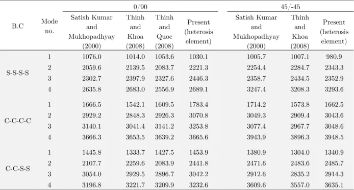
Table 6: Comparison of absolute natural frequencies of a laminated plate with bidirectional stiffeners.

2 layers (45/-45) 8 layers (45/-45/45…)

b/h Present _{results CFS (Reddy and}

Phan, 1985)

Present results _{CFS (Reddy and}

Phan, 1985)

9-NHE 9-NLE 8-NSE 9-NHE 9-NLE 8-NSE

5 10.335 10.244 10.243 10.335 12.892 12.863 12.862 12.892

10 13.044 12.975 12.975 13.044 19.289 19.235 19.235 19.289

20 14.179 14.154 14.153 14.179 23.259 23.225 23.225 23.259

25 14.338 14.322 14.321 14.338 23.924 23.899 23.899 23.924

50 14.561 14.557 14.556 14.561 24.909 24.902 24.901 24.909

(16)

Similar to the comparative analysis carried out for an unstiffened plate, the studies are further extended to a laminated plate with centrally placed bidirectional stiffeners under various edge con-ditions and the results are tabulated in Table 6 along with those available in the literature (Satish Kumar and Mukhopadhyay, 2000; Thinh and Khoa, 2008; Thinh and Quoc, 2008). The geometric and material properties of the stiffened plate are similar to the case 3.3.1. The comparison of results establishes the correctness of the mass matrix formulation for both the plate as well as the stiffen-ers.

3.3.3 Buckling Characteristics of Unstiffened/Stiffened Plates

For the buckling analysis, as in Eqs 36 and 37, one more matrix called geometric stiffness matrix appears in the formulation of the problem. It is essential to validate the formulation of such matrix.

In this regard, a non-dimensional quantity η (load bandwidth ratio) is introduced, which is either

the ratio of the position of the concentrated load to the width of the plate or width of edge com-pression to the width of the plate [refer Figures 3, 5 and 6]. The critical loads for an unstiffened

plate under concentrated load [see Figure 3(a)] are found for η = 0.25 and 0.5 and compared in

Table 7 with those available in the literature (Deolasi et al., 1995; Leissa and Ayoub, 1988). Simi-larly, a comparative study has been carried out for an S-S-S-S edged laminated plate with partial

in-plane load [see Figure 3 (b)] for various η and ply-orientations as shown in Figure 4. The

non-dimensionalised critical loads are validated with the results given by Sundaresan et al. (1998). It is

to be noted here that  is the critical load for a fully loaded plate and cr is the critical load for a

partially loaded plate.

Further, the buckling behaviour of S-S-S-S edged plate with a central single stiffener under

uni-formly distributed edge load over width b is studied for different bending rigidity of the stiffener.

The value of is varied from 0.05 to 0.20, and that of from 5 to 15. The results are presented in

Table 8 in non-dimensionalised form as 2 ( 2 )

cr P b /cr D

   , and compared with the classical solution

of Timoshenko and Gere (1961), numerical solutions of Mukhopadhyay and Mukherjee (1990), and Hamedani and Ranji (2013). In all the cases, the present results agree well with those available in the literature confirming the correctness of the geometric stiffness matrix for the plate as well as the stiffeners.

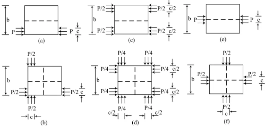
P P

c

(a)

P/2 c/2

(b)

P/2 P/2

P/2 b

c/2

b

(17)

a/b η Leissa and Ayoub (1988) Deolasi et al. (1995) Present

0.5 0.25 38.282 37.608 37.249

0.50 30.061 29.852 29.630

1.0 0.25 37.000 36.405 36.316

0.50 25.814 25.720 25.658

2.0 0.25 36.954 36.832 36.659

0.50 26.523 28.851 28.690

Table 7: Non-dimensionalised critical loads cr for S-S-S-S edged isotropic

plate under concentrated load [Figure 3 (a)].



(+0/-0) 23.38 (23.38) (+15/-15) 25.22 (25.22) (+30/-30) 32.04 (32.05) (+45/-45) 35.79 (35.80) (+60/-60) 29.90 (+75/-75) 15.70 (+90/-90) 10.46 (isotropic) 3.61 (3.61) - - - -Sundaresan et al.(1998)

0 10 20 30 40 50 60 70 80 90 100 110 0.0

0.5 1.0 1.5 2.0 2.5 3.0 3.5 4.0

2 2 2 2 22 2

P/2 c/2 P/2 P/2

P/2 b

c/2



/

cr

% of loaded edge length

Figure 4: Comparison of  /cr with % of edge load length for various angle-plies unstiffened

square plate with uniaxial partial in-plane loading from both the edges [Figure 3 (b)].

β δ

Non-dimensional buckling load

Neglecting T and e Considering T and e

Timoshenko and Gere (1961)

Mukhopadhyay and Mukherjee (1990)

Jafarpour and Ranji (2013)

Present (heterosis)

Jafarpour and Ranji (2013)

Present (heterosis)

5

0.05 12.00 11.72 11.89 11.80 11.91 11.86

0.10 11.10 10.93 11.08 10.98 11.09 11.27

0.20 9.72 9.70 9.85 9.69 9.86 10.01

10

0.05 16.00 16.00 16.01 15.97 18.16 17.91

0.10 16.00 16.00 16.01 15.97 16.97 17.20

0.20 15.80 15.44 15.01 15.67 15.04 15.77

15

0.05 16.00 16.00 16.01 15.97 20.41 20.30

0.10 16.00 16.00 16.01 15.97 20.41 20.33

0.20 16.00 16.00 16.01 15.97 19.36 20.33

T and e = Torsional rigidity and eccentricity of the stiffener

(18)

3.4 Convergence Study

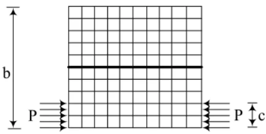
In the finite element method, it is essential to appropriately discretize the structure for proper

con-vergence of results. In this regard, the plate is discretized into m, number of rows and n, number of

columns, i.e. m x n plate elements as shown in Figure 5. Table 9 shows the convergence of the

non-dimensional critical loads for an unstiffened/stiffened plate under the action of uniaxial compressive edge load from one edge. The Table 9 also shows the non-dimensional vibration frequencies under

the action of in-plane edge loads P/Pcr = +0.5 (compressive) and P/Pcr = 0 (no in-plane load). It is

observed that the convergence of results is satisfactory for the mesh size of 10 x 10 and hence this mesh size is maintained throughout the work.

c b

P P

Figure 5: Laminated plate with centrally placed single stiffener along x-axis and load from one edge.

η

Mesh order m x n

Un-stiffened plate Stiffened plate

Buckling load (cr)

[ P/Pcr ] frequency (ϖ) Buckling

load (cr)

[ P/Pcr ] frequency (ϖ)

0 0.5 0 0.5

0.5 4 x 4 28.68 17.80 12.91 68.39 29.35 22.03

6 x 6 28.55 17.78 12.90 67.11 29.16 21.89

8 x 8 28.54 17.78 12.90 66.84 29.12 21.87

10 x 10 28.53 17.78 12.90 66.76 29.12 21.87

12 x 12 28.53 17.78 12.90 66.75 29.12 21.87

1.0 4 x 4 32.10 17.80 12.59 97.59 29.35 20.78

6 x 6 32.06 17.78 12.57 97.19 29.16 20.64

8 x 8 32.05 17.78 12.57 95.96 29.12 20.62

10 x 10 32.04 17.78 12.57 95.90 29.12 20.61

12 x 12 32.04 17.78 12.57 95.89 29.12 20.61

Table 9: Convergence of buckling load (cr) and frequency parameters (ϖ) for an S-S-S-S edged

angle-ply (+30o_/-30o₎₂_{square plate with/without central stiffener ( = 0.1 and = 10).}

3.5 Vibration and Buckling Behaviour of Laminated Stiffened Plate under Variety of Partial Edge Loading

(19)

For buckling analysis, an initial pre-buckling stress field has to be determined where the total load,

P acting on the plate is constant irrespective of the type and width of loading. Also, the total

vol-ume of stiffened plate is same irrespective of the number of stiffeners in any directions.

P c (a)

P b

P/2 c/2

(c) P/2 P/2 P/2 b c/2 P (e) P b _c P/2 c (b) P/2 b

P/4 c/2

(d) P/4 P/4 P/4 b c/2 P/2 P/2 b c P/2 P/2 c P/4 P/4 P/4 P/4 c/2 c/2 P/2 P/2 c (f)

Figure 6: Simply supported/clamped stiffened plates subjected to various loading cases: (a) Partial edge load from one edge; (b) Partial edge load from two adjacent edges; (c) Partial edge load from two opposite edges; (d) Partial edge load from all the corners; (e) Partial edge load from the center, unidirectional; (f) Partial edge load from the center, bidirectional.

3.5.1 Vibration Characteristics of Laminated Stiffened Plate under Uniaxial Edge Loading

The effect of non-dimensional load λ on the vibration behaviour of S-S-S-S edged laminated square

plate with a centrally placed single stiffener has been studied for = 0.1 and = 10. This load case is shown in Figure 6 (a). The results presented in Figures 7 (a) and (b) indicate that the frequency decreases with an increase in the value of edge load. As the load approaches the critical value, the vibration frequency reduces to zero and this load is called the buckling load. This dynamic method of analysis overcomes the shortcomings of the evaluation of critical loads by the static approach, which generally happens where the in-plane stress distribution within an element is significantly non-uniform. This method of analysis has been adopted to determine the critical loads for various problems discussed henceforth.

0 10 20 30 40 50 60 70 80 90 100 0 5 10 15 20 25

30 

0.0 P c P b (a) 0.4 No n-d ime ns iona l f req uen cy (  )

Non-dimensional load (  0.6 0.8 1.0 0.2

0 5 10 15 20 25 30 35 40 45 50 55 0 2 4 6 8 10 12 14 16 18 20 22 24 26 28 30 32

= 0.2

P c P b (b) N on-di m en si on al fr eque nc y (  )

Non-dimensional load (  angle (+0/-0) (+15-15) (+30-30) (+45-45) (+60-60) (+75-75) (+90-90) 2 2 2 2 2 2 2

(20)

3.5.2 Laminated Stiffened Plate under Uniaxial and Biaxial Partial Edge Load from One Edge

The effect of a four layered anti-symmetric ply-orientation (±θo)2 and the load bandwidth ratio η on

the stability behaviour of a unidirectional loaded square plate with a central single stiffener [refer Fig-ure 6 (a)] for S-S-S-S and C-C-C-C edged stiffened plates are depicted in FigFig-ures 8 (a) and (b), re-spectively. It is noticed from Figure 8 (a) that the buckling resistance is generally found to be

maxi-mum for a plate with (±30o)2 layup irrespective of the values of η. This may be attributed to the

higher flexural stiffness of the anti-symmetric stiffened plate with (±30o)2 layup. Similarly, it is

no-ticed from Figure 8 (b) that the critical load is found to be maximum for ply-orientations between

(±30o)2 and (±40o)2 depending on values of η for the C-C-C-C edged stiffened plate. From these two

figures, it is also inferred that the buckling load generally increases with increase in the value of η.

This may be due to the fact that the contribution of the stiffener in resisting critical load increases as the line of action of the resultant load approaches the stiffener center line. It may be stated that the

stiffened plate with around (±30o)2 layup can be a better choice for this type of loading condition.

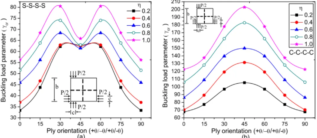
Similar studies are carried out for the same plate with biaxial edge loading and centrally placed biaxial stiffeners [refer Figure 6 (b)] and the results are depicted in Figures 9 (a) and (b). In Figure 9 (a), it is noticed that the buckling load steadily increases to a maximum as the ply-orientation

varies from (±0o)2 to (±30o)2 and starts decreasing from (±30o)2 to (±45o)2. As the value of

ply-orientation increases from (±45o)2 to (±60o)2, the critical loads again continue to increase to their

maximum values. From (±60o)2 to (±90o)2, the critical loads are found to decrease to a minimum.

This wavy variation is symmetrical in nature and the maximum buckling values are found at both (±30o)2 and (±60o)2 ply-angles.

Similarly, it can be noticed in Figure 9 (b) that the critical loads monotonically increases as the

value of ply-orientation is increased from (±0o)2 to (±45o)2 and decreases from (±45o)2 to (±90o)2.

The decreasing trend of critical loads from (±30o)2 to (±45o)2 to an intermediate value as observed

in Figure 9 (a) is not reflected in this case, i.e. wavy variation does not exist in the C-C-C-C edged stiffened plate. It may be attributed to the fact that the edge rotational restraint increases the stiff-ness of the stiffened plate predominantly and hence the critical loads continue to increase for all

values of η as seen in Figure 9 (b). For this kind of loading, the stiffened plate with (±30o)2 or

(±60o)2 layup may be more useful for S-S-S-S edge conditions and the stiffened plate with (±45o)2

layup may be a better choice for C-C-C-C edge conditions.

0 15 30 45 60 75 90

0 10 20 30 40 50 60 70 80 90 100

0 15 30 45 60 75 90

30 40 50 60 70 80 90 100 110 120 130 140 150 160 170 180 190 200

(a)

S-S-S-S

Bu

ck

lin

g

load

p

ar

am

et

er

cr

)

Ply orientation (+/+/-)



0.2 0.4 0.6 0.8 1.0

P c P

b

C-C-C-C

P c P

b

C-C-C-C

(b)

Bu

ck

lin

g

lo

ad

p

ar

am

ete

r

cr

)

Ply orientation (+/+/-) 

0.2 0.4 0.6 0.8 1.0

Figure 8: Variation of cr with different ply-orientation (a) for simply supported and (b) for clamped square plate

(21)

0 15 30 45 60 75 90 30

35 40 45 50 55 60 65 70 75 80

0 15 30 45 60 75 90 60

70 80 90 100 110 120 130 140 150 160 170 180 190 200 210

(a)

S-S-S-S 

Bu

ck

lin

g l

oad

p

ar

am

et

er

cr

)

Ply orientation (+/+/-) 0.2 0.4 0.6 0.8 1.0

P/2 c P/2

b P/2

P/2 c

P/2 c P/2 b

P/2

P/2 c

(b)

C-C-C-C

Bu

ck

ling

load

para

m

et

er

cr

)

 0.2 0.4 0.6 0.8 1.0

with central orthogonal stiffeners ( = 0.1 and = 10) under bidirectional partial edge loading from one edge.

3.5.3 Laminated Stiffened Plate under Uniaxial and Biaxial Partial Edge Loading from Both Edges

The effect of load case shown in Figure 6(c) on the critical loads of unidirectional stiffened plate is examined and the results are depicted in Figures 10 (a) and (b) for different ply-orientations and

boundary conditions (S-S-S-S, C-C-C-C). The buckling load is found to be maximum at (±30o)2

layup irrespective of the values of η as can be seen in Figure 10 (a). The same phenomenon has

been observed in Figure 8 (a), the possible reason being that the effect of loading from one edge [Figure 6 (a)] holds true for loading from both edges [Figure 6(c)]. Further, it is interesting to

men-tion that for a particular ply-angle of about ( 48o)2, the critical loads are practically same

irrespec-tive of the values of η, and similar phenomenon is again observed at ( 90o)2 ply-angle in Figure 10

(a). The buckling behaviour of C-C-C-C edged stiffened plate, as shown in Figure 10 (b), is almost similar to that of S-S-S-S edged stiffened plate. However, in this case, the critical loads are

inde-pendent of the value of η for only one particular ply-orientation, i.e. at ( 90o)2.

The variation of critical loads for the bidirectional loaded square plate with bidirectional stiffen-ers [refer Figure 6 (d)] is now investigated and the results are presented in Figures 11 (a) and (b) for S-S-S-S and C-C-C-C edge conditions, respectively. The wavy variation of buckling loads ob-served in Figure 11 (a) is similar as that obob-served in Figure 9 (a). In both the cases, it is obob-served

that the curves have two peaks, i.e. at (±30o)2 as well as (±60o)2 layups. Therefore, it is appropriate

to choose the stiffened plate with either of these layups for these types of loading cases. The buck-ling variation of a stiffened plate with C-C-C-C edge condition is shown in Figure 11 (b). The varia-tion is slightly different when compared to the one shown in Figure 9 (b). In this case, the curves

for η = 0.2 to 0.6 have double peaks, i.e. at (±30o)2 and (±60o)2 ply-angles and beyond η = 0.6, the

curves are having a single peak at (±45o)2 angle. However, in this case, the choice of

ply-orientation is purely dependent on the width of edge compression. For this type of loading, the

stiff-ened plate with (±45o)2 layup may be suitable for η = 0.8 – 1.0, whereas, for the remaining values

(22)

0 15 30 45 60 75 90 20 30 40 50 60 70 80 90 100 110

0 15 30 45 60 75 90 50 60 70 80 90 100 110 120 130 140 150 160 170 180 190 200 210 (a) Bu ck lin g loa d par am et er cr ) S-S-S-S

Ply orientation (+/+/-)  0.2 0.4 0.6 0.8 1.0 P/2 c/2 P/2 P/2 P/2 b c/2 P/2 c/2 P/2 P/2 P/2 b c/2 (b) C-C-C-C Bu ck ling load pa ra m et er cr )

 0.2 0.4 0.6 0.8 1.0

Figure 10: Variation of cr with different ply-orientation (a) for simply supported and (b) clamped square plate with

centrally placed single stiffener ( = 0.1 and = 10) under unidirectional partial edge loading from both edges.

0 15 30 45 60 75 90 50 55 60 65 70 75 80 85 90 95 100 105

0 15 30 45 60 75 90 110 120 130 140 150 160 170 180 190 200 210 (a) S-S-S-S

Ply orientation (+/+/-)  0.2 0.4 0.6 0.8 1.0 Bu ckling loa d parameter cr ) P/4c/2 P/4 P/4 P/4 b c/2 P/4 P/4 P/4 P/4 c/2 c/2 (b) P/4c/2 P/4 P/4 P/4 b c/2 P/4 P/4 P/4 P/4 c/2 c/2 C-C-C-C Buckli

ng load p

aram

ete

r

cr

)

 0.2 0.4 0.6 0.8 1.0

with centrally placed orthogonal stiffeners ( = 0.1 and = 10) under bidirectional partial edge load from both edges.

3.5.4 Laminated Stiffened Plate with Uniaxial and Biaxial Partial Edge Loading at the Center

The variation of cr with the ply-orientation angles (±θo)2 for S-S-S-S and C-C-C-C square plate

with a centrally placed single stiffener subjected to uniaxial loading [refer Figure 6 (e)] is shown in

Figures 12 (a) and (b). It is noticed from Figure 12 (a) that, in general, the critical load cr is

max-imum for a ply-angle of (±30o)2 except for lower values of η. Further, the variation of buckling load

after (±55o)2 ply-orientations is not significant with respect to η. Similar behaviour can also be

ob-served in a C-C-C-C edged stiffened plate as shown in Figure 12 (b). However, in this case, the

buckling variation is not significant after (±75o)2 ply-orientation for all values of η.

Similar studies are carried out for the same plate with a centrally placed biaxial stiffener and biaxial loading conditions and the results are depicted in Figures 13 (a) and (b). The study

indi-cates that the critical load generally increases with an increased value of η. It may be due to