J. of the Braz. Soc. of Mech. Sci. & Eng. Copyright 2006 by ABCM October-December 2006, Vol. XXVIII, No. 4 /505
Luciano L. Menegaldo
Member, ABCM [email protected] Military Institute of Engineering - IME Dep. of Mechanical and Materials Engineering 22290-270 Rio de Janeiro, RJ. Brazil
Rogerio Eduardo S. Santana
[email protected] Escola Politécnica, University of São Paulo Mechanical Engineering Department 05508-900 Sao Paulo, SP. BrazilAgenor de Toledo Fleury
Emeritus Member, ABCM[email protected] FEI University Center Mechanical Engineering Department 09850-901 São Bernardo do Campo, SP. Brazil and Escola Politécnica, University of São Paulo Mechanical Engineering Department
Kinematical Modeling and Optimal
Design of a Biped Robot Joint Parallel
Linkage
This paper shows the design and analysis of a parallel three-dimensional linkage, conceived to work as the ankle and hip joints of an anthropometric biped robot. This kind of mechanism architecture provides low-weight, highly stable assemblies, and allows the use of actuator synergies. On the other hand, the mechanical transmission ratio is not usually favorable, and a non-linear kinematic model has to be derived and solved. The mechanism proposed here is driven by two rotational servo-actuators, and allows the joint to follow a specified angular trajectory determined by the gait pattern. Namely, the joint linkage can generate dorsi/plantar flexion and inversion/eversion of the ankle, and hip flexion/extension and adduction/abduction movements. Several approaches to the direct and inverse kinematical modeling of the linkage are presented and compared, regarding their accuracy and computational cost, where the last performance parameter is closely related to on-line computer implementing of the controller. Strategies to fit current gait angular amplitudes into the linkage workspace, as well as singularity analysis, are discussed. An optimization method was applied to find some geometrical design parameters of the linkage that minimizes a cost function. This function is the mean transmission ratio between the motor inputs and the joint output torques over a predefined dominion. The minimization is constrained to a minimum workspace area value and to minimum and maximum values of the design parameters. Several design solutions were generated. The chosen was one where the workspace is compatible to the gait amplitude requirements and that exhibits the lowest cost function. A biped robot using the linkage geometry designed in this paper has been built and tested with real human gait data acquired in a gait lab.
Keywords: Parallel linkage, mechanisms, gait analysis, biped robot, optimal design
Introduction
1
In the recent years, a great amount of scientific and engineering research has been devoted to the development of legged robots able to reach gait patterns more or less similar to human beings. Towards this objective, many scientific papers have been published, focusing on different aspects of the problem. Some articles describes the overall design, control, mechanics and electronic issues of several robots being developed around the world (Shih, 1996; Sardain et al., 1998; Hirai et al., 1998; Yamaguchi et al., 1999; Sagakami et al., 2002; Buss et al., 2003; Kin et al. 2004; Azevedo et al., 2004). The robots found in these and other papers are usually built as active kinematic chains driven by electrical motors or linear actuators, present from 2 to 17 degrees of freedom, their joints are directly driven by the motors, in most of the cases, or use linkages to transmit movements. Some robots have trunk and arms, to aid the achievement of stable gaits through static or dynamic compensation approaches (the well-known ZMP Zero Moment Point, for example), while others have only the lower limbs. Other papers, instead of describing the whole engineering approaches, address particular aspects of the problem, such as the generation of energy efficient limb trajectories seeking simultaneously for body stability (Bessonet et al., 2004), based on neural networks (Gonçalves e Zampieri, 2003), analytic expressions (Albert and Gerth, 2003) or nonlinear oscillators, mimicking the spine Central Pattern Generators neuronal circuitry (Aoi and Tsuchiya, 2005). A few papers however address the specific problem of designing, modeling and optimizing mechanical linkages that should be used in legged robot locomotion. Ogata and Hirose (2004) have presented a parallel ankle mechanism to be used in quadruped robots. Shieh et al (1997)
Presented at XI DINAME – International Symposium on Dynamic Problems of Mechanics, February 28th - March 4th, 2005, Ouro Preto. MG. Brazil. Paper accepted: June, 2005. Technical Editors: J.R.F. Arruda and D.A. Rade.
has shown the design and optimization of a one degree-of-freedom leg for an all-terrain walking machine.
This paper describes the kinematical modeling and design optimization of a parallel linkage used in a biped robot (Menegaldo et al., 2003; Santana, 2005). The linkage must transform the rotations and torques generated by a pair of DC servo-motors into robot’s ankle movements, namely foot plantar flexion / dorsiflexion and foot inversion / eversion, as well as hip flexion/extension and adduction/abduction. We have chosen a parallel linkage architecture that has a high stiffness, low weight and reasonable transmission ratio between the servo-motors and the end effector, i.e., the foot. Parallel mechanisms have been used by some authors in ankle and hip joints for biped robots (Sardain et al., 1998; Paluska, 2000; Azevedo et al., 2004). The mechanisms presented by these authors consist in two linear actuators built with rotary DC motors and screw-nuts. The actuators are assembled in a spatial mechanism with two parallel rod-crank systems, and used three universal (cardanic) and two spherical joints. This two degrees-of-freedom spatial mechanism is very robust and may provide a high torque with reasonable velocity and range-of-motion.
Here, we propose an alternative assembly to this mechanism, using low-cost commercially available rotational servo-actuators, usually used in RC airplanes and boats. In addition, four spherical joints and only one cardanic joint is used, then lowering the cost of the linkage components. The linkage drawing for ankle and hip, and an overall view of the robot is shown in Figures 1 and 2. If both servo bars rotate upward, the foot makes a plantar flexion. If they rotate downward, the foot does a dorsiflexion. If one bar rotates up and the other down, the foot may perform an inversion or an eversion. This class of linkages has an important advantage of using simultaneously the torque of two servo-actuators to perform the same movement. On the other hand, the relation between the servos and the joints angles is not trivial, and requires a kinematical model of the linkage.
are discussed, specially the allowable workspace size and shape and the transmission ratio. An optimization problem is then formulated to find the optimal dimensions of the linkage bars regarding the maximization of the transmission ratio, at the same time that a minimal workspace size works as optimization constraint. The achieved solutions are then compared to normal data from experimental gait analysis. The results, although not exhaustively explored, show that the achieved design parameters allow the construction of a linkage with a feasible workspace for normal gait. On the other hand, the increasing of the minimal workspace size led in the optimization process to the increase of the cost function value.
Figure 1. Ankle and Hip linkages.
Figure 2. Overall view of the robot.
Nomenclature
φ1 = inversion/eversion angle, degrees
α1,2 = servo angles, degrees
(xi, yi, zi) = local reference frame no. i
TM1, M2 = torques delivered by the servo-actuators 1 and 2, N.m Ta = vector of external torques applied in foot, N.m
Rij = rotation matrix from system i to j η = cost function, dimensionless W = workspace size, dimensionless
Jx = Jacobian matrix with relation to φ = [φ1, φ2]
Jq = Jacobian matrix with relation to α = [α1, α2]
A, B, C, L2: dimensional parameters, m
Linkage Kinematics
After the linkage architecture has been selected, the detailed design and optimization requires the development of a kinematic mathematical model. Such a model is called direct kinematic model when one wants to find the final configuration of the linkage as a function of the input or of the generalized coordinates. Here, we look for finding the foot angles (inversion/eversion φ1 and ankle
plantar flexion/extension φ2) as a function of the both servo angles
α1 and α2. Direct kinematics is useful for design and computer animation purposes. However, for control purposes, it is necessary to have an inverse kinematics expression that allows one to find the α1,2 servo angles as a function of φ1,2. These are the variables where
the gait kinematics is usually expressed. The linkage position analysis for both direct and inverse kinematic problems will be addressed bellow. The modeling process is the same for the design of the hip joint linkage, and therefore the development shall be made only for the ankle.
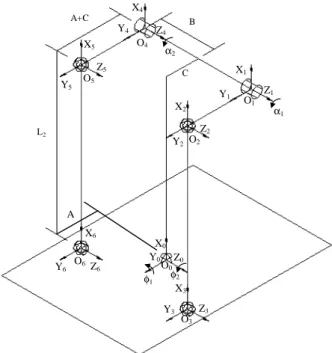
Observing Figure 3, the ankle reference frames O0-x0y0z0 (base),
O1-x1y1z1 and O4-x4y4z4 are fixed to the same rigid body, the robot
shank shaft. The reference frames O3-x3y3z3 and O6-x6y6z6 are in the
foot platform, while frames O2-x2y2z2 and O5-x5y5z5 are, in turn,
fixed to the bars connected to the actuators.
A+C
L2
B
C
X0
Y0 Z0
X1
Y1 Z1
X2
Y2
Z2
X3
Z3
Y3
X4
Z4
Y4
X5
Y5
Z5
X6
Z6
Y6
α2
α1
φ2
φ1
O4
O5
O1
O2
O6
O3
O0
A
J. of the Braz. Soc. of Mech. Sci. & Eng. Copyright 2006 by ABCM October-December 2006, Vol. XXVIII, No. 4 /507
The rotation matrix 3 0
R which transforms the base system O0
-x0y0z0 to O3-x3y3z3 can be calculated considering that the foot rotates
an angle φ2 around z0 and φ1 around y0. The successive rotations
give the transforming matrix:
( )
( )
( )
( )
( )
( )
( )
( )
( )
( )
( )
( )
1 2 1 2 1
3
0 2 2
1 2 1 2 1
cos cos cos sin sin
sin cos 0
sin cos sin sin cos
R
φ φ φ φ φ
φ φ
φ φ φ φ φ
⋅ − ⋅ = − ⋅ ⋅ (1)
The displacement vector O O0 3, expressed in the base reference
frame is given by
3 0 3 0
0
O O R A
B = ⋅ (2)
The rotation matrix 2 1
R that specifies the O2-x2y2z2 frame in
relation to O1-x1y1z1 is given by
( )
( )
( )
1( )
12
1 1 1
cos sin 0
sin cos 0
0 0 1
R α α α α − =
- (3)
Therefore, the coordinates of the System 2 (x2, y2, z2) origin, i.e.,
the vector
2 0O
O in the base reference frame, can be expressed by:
(
)
2 2 0 2 1
0
0
L
O O C R A C
B = − + ⋅ + (4)
The distance between the points O2 and O3 is the same as the bar
L2 length:
0 2 0 3 2
O O −O O =L (5)
Substituting Eqs. (2) and (4) in Eq. (5), a function relating the foot angles φ1 and φ2 to the servo angle α1 is found:
(
)
(
)
( )
(
)
( )
( )
( )
( )
( )
( )
( )
( )
(
)
( )
( )
(
)
( )
( )
(
)
( )
( )
( )
21 1 1 2 1
2 1 2
2
2 1 1
2 1 2 1 2
1 2 1 1 1 1 2
2 2
, , 0 2 cos
2 sin 2 cos
2 sin 2 cos
2 cos sin 2 sin sin
2 cos cos
2 sin sin
2 sin cos sin
2 2 2 2
f C A C
L A C A C
B L B
A L A B
A A C
B A C
A A C
C A C B
α φ φ α
α φ
φ φ
φ φ φ φ
α φ
α φ
α φ φ
= = − ⋅ + ⋅ ⋅ − ⋅ ⋅ + ⋅ + ⋅ ⋅ ⋅ − ⋅ ⋅ ⋅ − ⋅ ⋅ + ⋅ ⋅ ⋅ ⋅ − ⋅ ⋅ ⋅ ⋅ − ⋅ ⋅ + ⋅ ⋅ + ⋅ ⋅ + ⋅ ⋅ − ⋅ ⋅ + ⋅ ⋅ ⋅
+ ⋅ + ⋅ ⋅ + ⋅ + ⋅A2
(6)
For the opposite kinematic chain, if one uses the same reasoning, the relationship between
φ
1 andφ
2 and the other servo angleα
2 can be established as:(
)
(
)
( )
(
)
( )
( )
( )
( )
( )
( )
( )
( )
(
)
( )
( )
(
)
( )
( )
(
)
( )
( )
( )
22 2 1 2 2
2 2 2
2
2 1 1 2 1 2
1 2 2 2 2 1 2 1 2
2 2
, , 0 2 cos
2 sin 2 cos
2 sin 2 cos 2 cos sin
2 sin sin
2 cos cos
2 sin sin
2 sin cos sin
2 2 2 2
f C A C
L A C A C
B L B A L
A B
A A C
B A C
A A C
C A C B
α φ φ α
α φ
φ φ φ φ
φ φ
α φ
α φ
α φ φ
= = − ⋅ + ⋅ ⋅ − ⋅ ⋅ + ⋅ + ⋅ ⋅ ⋅ + ⋅ ⋅ ⋅ − ⋅ ⋅ + ⋅ ⋅ ⋅ ⋅ + ⋅ ⋅ ⋅ ⋅ − ⋅ ⋅ + ⋅ ⋅ − ⋅ ⋅ + ⋅ ⋅ − ⋅ ⋅ + ⋅ ⋅ ⋅
+ ⋅ + ⋅ ⋅ + ⋅ + 2
A
⋅
(7)
Inverse Kinematics
The inverse kinematic problem consists in finding the servo angles α
1,2 that generates the desired foot angles φ1,2. Equation (6)
can be solved for α
1 by considering:
( )
( )
1 sin 1 2 cos 1 3 0
a ⋅ α +a ⋅ α +a = (8)
where:
(
)
( ) (
)
( )
( ) (
)
1 2 1
1 2
2 2 sin
2 cos sin
a L A C B A C
A A C
φ
φ φ
= − ⋅ ⋅ + + ⋅ ⋅ ⋅ +
− ⋅ ⋅ ⋅ ⋅ +
(
2)
( ) (
)
2 2 2 cos 2
a = − ⋅ C + ⋅A C − ⋅ ⋅A φ ⋅ A+C
( )
( )
( )
( )
( )
( )
( )
2
3 2 2 1 1
2 1 2 1 2
2 2 2
2 cos 2 sin 2 cos
2 cos sin 2 sin sin
2 2 2 2
a A C B L B
A L A B
A B C A C
φ φ φ
φ φ φ φ
= + ⋅ ⋅ ⋅ − ⋅ ⋅ ⋅ − ⋅ ⋅ + ⋅ ⋅ ⋅ ⋅ − ⋅ ⋅ ⋅ ⋅ + ⋅ + ⋅ + ⋅ + ⋅ ⋅
Then one may use the following change of variables:
2 2 1 2 1 1 1 ) cos( 1 2 ) sin( t t t t + − = + = α α
where
= 2 tan α1
t
Eq. (8) is then rewritten as:
(
)
2 2 1(
3 2)
02
3−a ⋅t + ⋅a ⋅t+ a +a = a
(9)
This is a 2nd order algebraic equation in t, that after solved and transformed back to α1 gives:
2 3 2 3 2 2 2 1 1 1 2 a a a a a a arctg − − + ± − ⋅ =
α
(10)(
)
( ) (
)
( )
( ) (
)
1 2 1
1 2
2 2 sin
2 cos sin
b L A C B A C
A A C
φ
φ φ
= − ⋅ ⋅ + − ⋅ ⋅ ⋅ +
− ⋅ ⋅ ⋅ ⋅ +
(
2)
( ) (
)
2 2 2 cos 2
b = − ⋅ C + ⋅A C − ⋅ ⋅A φ ⋅ A+C
( )
( )
( )
( )
( )
( )
( )
3 2 2 1
2
1 2 1 2
1 2 2 2 2
2 cos 2 sin
2 cos 2 cos sin
2 sin sin
2 2 2 2
b A C B L
B A L
A B
A B C A C
φ φ
φ φ φ
φ φ
= + ⋅ ⋅ ⋅ + ⋅ ⋅ ⋅ − ⋅ ⋅ + ⋅ ⋅ ⋅ ⋅ + ⋅ ⋅ ⋅ ⋅
+ ⋅ + ⋅ + ⋅ + ⋅ ⋅
Direct Kinematics
The solution given byEquations (10) and (11) is suitable for control purposes, as the foot angle is controlled through the servo angles. On the other hand, if the servo angles are known and the foot angles must be found, e.g., for generating a computer graphical animation, designing, or providing information to a hierarchical controller, both equations (6) and (7) shall be solved simultaneously, as a non-linear algebraic system. The system has been solved with Least-Squares algorithms (Matlab fsolve function) or Newton methods (Santana, 2005), and the results are very similar. An alternative solution, that uses interpolating polynomials, gives faster answers, suitable for real-time applications:
2 2
1 1 2 1 3 2 4 1 5 2 6 2 1 2 2
2 1 2 1 3 2 4 1 5 2 6 2 1
a a a a a a
b b b b b b
φ α α α α α α
φ α α α α α α
= + ⋅ + ⋅ + ⋅ + ⋅ + ⋅ ⋅
= + ⋅ + ⋅ + ⋅ + ⋅ + ⋅ ⋅ (12) By varying the foot angles −15o≤ ≤φ1 15o and −15o≤φ2≤15o, with
0.5o step-size, the servo α1,2 angles are found through the inverse
kinematic problem, that is through solving Equations (10) and (11). Collecting a series of n solutions and arranging them in matrix-form:
( ) ( ) ( ) ( ) ( ) ( )
( ) ( ) ( ) ( ) ( ) ( )
( )
( )
2 2
1 1
1 2 1 2 2 1
2
3
4
5
2 2 1
6
1 2 1 2 2 1
1
1 1,1 1, 2 1,1 1,2 1,2 1,1
.
. . . .
.
. . . .
.
. . . .
.
. . . .
1 ,1 ,2 ,1 ,2 ,2 ,1
x A
a a a a a
n a
n n n n n n
φ
α α α α α α
φ
α α α α α α
⋅
⋅ =
⋅
B
(13)
The non-square linear system may be solved through the pseudo-inverse matrix:
(
t)
1 tx= A ⋅A − ⋅A ⋅B (14)
where the At is the transpose of matrix A.
The same procedure is used to find the b coefficients that fit the flexion/extension angles as a function of the servo angles. The three solutions, namely, Least Squares, Newton and Polynomials, have been implemented with very similar results. As it should be expected, the third method gives much faster results when compared to Matlab fsolve and Newton methods. The same analysis is performed to find the kinematical model of the hip. In this case, the mechanism should be reversed, and the thigh substitutes the foot in the former analysis. The movements are the flexion-extension of the thigh, in the saggital plane, and adduction-abduction in the frontal one. The “fixed” part of the hip linkage, to where the two servos are attached, is no longer the calf, as in the case of the ankle, but now the bar that connects the two legs, i.e., the “pelvis”.
Workspace Analysis
The proposed linkage must generate the joint angle limits usually observed in normal gait. Nevertheless, the dimensions of the linkage constitutive elements strongly influence the shape and the size of the workspace. One of the constraints is that the solution of equations (6) and (7) must have only real parts. Varying the ankle angles in the interval
1 90o φ 90o
− ≤ ≤ and −90o≤φ2≤90 1 step - sizeo o
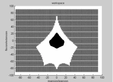
one can find the region of the domain where both α1 and α2 are real. Figure 4 has been generated with the dimensions of a linkage prototype with A=55.3 mm, B=68.4 mm and L2=34.2 mm.
On the other hand, the spherical joints used to assembly the mechanism (TB 1/4” PFD, Termicom S. A., São Paulo, Brazil) allows only a limited amount of angular displacements, namely ± 21º in each direction. These angular displacements impose restrictions to the robot movements which are expressed by the limits:
1 25o φ 25o
− ≤ ≤ and −25o≤φ2≤25 0.5 step - sizeo o
If the values of the angles of the four joints are inside the allowable limits, the solution is considered as valid. In Figure 4, the white region corresponds to the solutions obtained from the first test (only real solutions), and the darker from the second (spherical joint limits).
Figure 4. Workspace for a particular set of linkage dimensions. The white region corresponds to the real solutions of the linkage kinematic model, and the darker the workspace where the spherical joints are inside their angular displacement limits.
Linkage Optimal Design
The objective of the linkage optimal design is to find the best arrangement of the A, B, C and L2 robot dimensions such that the
torque is maximally transmitted between the servos and the foot. However, as inequality constraints, these parameters must not exceed maximum mechanical construction limits. The optimization problem can be formulated as minimizing the cost function η:
If the solution of the kinematical model is real and relative angles of the bars joined with spherical joints do not exceed the constructive constraints, the parameter λ is computed for this particular point as:
t 2 2 M 2 1 M i
T T
i i
J. of the Braz. Soc. of Mech. Sci. & Eng. Copyright 2006 by ABCM October-December 2006, Vol. XXVIII, No. 4 /509
where n is the number of points of the discretized domain where λi
has been evaluated for a given feasible pair φ1 and φ2. TM1 and TM2
are the torques delivered by the servo-actuators and Ta is a vector of the torques applied in foot or pelvis Ta = [Tφ1 Tφ2]t.
The [φ1, φ2] limits for this domain have been fixed inside the interval [-25o, 25o]. To evaluate λ, Equations (6) and (7) must be
differentiated with relation to time.
0 0 0 0 2 2 2 1 1 2 2 2 2 1 1 2 2 2 2 1 1 1 1 2 2 1 1 1 1 1 = ⋅ + ⋅ + ⋅ + ⋅ ⇒ = = ⋅ + ⋅ + ⋅ + ⋅ ⇒ = dt d d df dt d d df dt d d df dt d d df dt df dt d d df dt d d df dt d d df dt d d df dt df
α
α
α
α
φ
φ
φ
φ
α
α
α
α
φ
φ
φ
φ
(17)By defining the Jacobian matrices Jx and Jq and the vectors
[
]
T2 1 φ
φ
φɺ= ɺ ɺ and
[
]
T 2 1 αα αɺ= ɺ ɺ
= = 2 2 1 2 2 1 1 1 2 2 1 2 2 1 1 1
α
α
α
α
φ
φ
φ
φ
d df d df d df d df J d df d df d df d dfJx q (18)
the following relation is found:
(
1)
x q x q
Jφɺ=Jαɺ → φɺ= J −J αɺ (19) It can be shown (Craig, 1986) that for the torques, the above equation can be written as:
(
)
= − 2 1 1 2 1 φ φ T T J J T T T q x M M (20)For all the simulated tests, unitary torque values were considered for Ta. In addition, the minimizing of the cost function (15), evaluated from eqs. (16) and (20), is constrained to minimal and maximum values of the design parameters as well as constrained to the limits of the Workspace (W):
max max max min max 2 2 min 2 min L , C , A A A A C C C L L L W W : that such min 2 ≤ ≤ ≤ ≤ ≤ ≤ ≥ η
The Workspace (W) is evaluated as the ratio of the total number of points of the discretized domain (m) to the number of valid points, n.
Results
Three solutions have been investigated for the linkage optimal design. In the first, the dimensional parameters of a linkage prototype (Menegaldo et al., 2003) are used to find reference values for W and η. For the second and the third solutions, the first one is used as the initial guess for the optimization routine (Matlab fmincon). In the second case, the workspace W has been fixed as W=0.3 and in the third, W=0.25. The optimized parameters as well as the values of the objective function η and the achieved workspace W are shown in Table 1. The B parameter was fixed in 68.4 mm for
all cases. Each solution took around 10 minutes CPU time using a Pentium III 600MHz PC Desktop.
Table 1. Linkage bar dimensions, workspace size and cost function obtained from the solution of the optimization problem. The Solution 1 was found heuristically, and used to build the first linkage prototype.
Solution A (mm) C (mm) L2 (mm) W ηηηη
1 60 0 34 0.226 0.659
2 60 3 62 0.25 0.691
3 60 11.2 70 0.3 0.784
To verify if the obtained linkage designs are able to reach the joint angles usually observed in normal human gait, real data from gait lab analysis (from Normative Database of AACD – Associação de Assistência à Criança Defeituosa, São Paulo, Brazil) have been plotted over the workspace diagram of the solutions. Mean gait data from AACD Vicon System, namely foot plantar flexion / dorsiflexion and foot inversion / eversion, as well as hip flexion/extension and adduction/abduction have been plotted over a linkage workspace analysis diagram. The workspaces obtained for solutions 2 and 3 (white area), superposed to the real gait trajectories are shown in Figure 5. Part of the figure is printed with “x”, points corresponding to the linkage workspace where the angles of the spherical joints exceed the maximum constructive angle of 21o, i.e., where the λ
parameter of Eq. (16) is evaluated. Solution 2 is designed to present a smaller admissible workspace than Solution 3, with a resulting smaller cost function and a better transmission ratio. However, as one can observe from Figure 5 (up), the joint angles required to perform a normal gait cycle will not be reached for some angular positions, where the continuous line crosses the “x” printed region. When the workspace is augmented to W=0.30 (down), the transmission ratio is worse, but the all the gait cycle positions can be achieved by the linkage, both for hip and ankle movements.
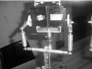
Figures 6 and 7 show the ankle and hip mechanisms as built in the biped robot. The robot components have been machined in Al alloys at IPT (Sao Paulo State Institute for Technological Research). The universal joint was specified as DIN 808-G (Imetex, Sao Paulo, Brazil), with 16mm of diameter and 34mm of total length. The chosen servo-actuators were the ones that presented the best maximum torque among the available for RC applications, the HOBBICO CS-80 (maximum torque of 2.4 N.m). The built robot has been tested with real gait data and has been able to reproduce normal and pathological gait patterns. For more details on the robot’s mechanical and electronic parts, sensors and testing, one may see Santana (2005). Inverse kinematics equations have been included on the robot control software, written in C language, to drive a microcontrolled board able to deliver a Pulse Width Modulated (PWM) signal proportional to each of the servo angles α.
Discussion
-25 -20 -15 -10 -5 0 5 10 15 20 25 -25
-20 -15 -10 -5 0 5 10 15 20 25
inversion/evers ion
fl
e
x
io
n
/e
x
te
n
s
io
n
-25 -20 -15 -10 -5 0 5 10 15 20 25
-25 -20 -15 -10 -5 0 5 10 15 20 25
inversion/evers ion
fl
e
x
io
n
/e
x
te
n
s
io
n
Figure 5. Workspace and gait trajectories for Solution 2 (up) and Solution 3 (down). The continuous line is the hip angular displacements in one gait cycle, and the dashed line the ankle. “x” marked region corresponds to linkage positions where the maximum spherical joint anlgle exceedes the construtive limits.
Figure 6.Posterior view of the ankle linkage.
Figure 7. Anterior view of the hip linkage.
Computation of the objective function value for the built prototype (Solution 1) has shown that the torque transmission ratio relationship for this particular solution is good, when compared to the optimized solutions. However, Solution 1 is not able to reach all the workspace points required for normal gait. The optimization approach has shown that the workspace size should be controlled by defining a constraint Wmin. Nevertheless, the increasing of the
workspace size has led to a less-efficient solution from the torque transmission ratio point of view, as can be observed in Table 1.
Solution 2 is acceptable, although gait trajectory trespasses the allowable limits of linkage operation in some few regions. If a small reduction in joint amplitude is acceptable for some particular robot application, the geometry obtained from Solution 2 should be used. On the other hand, if gait trajectory must be followed in all the span of the real gait data used, Solution 3 should be the most appropriate choice. The cost function η is an estimator of the overall transmission ratio of the linkage. Although this ratio is variable along the workspace, the estimator seems to be a good indicative design index.
A prototype with the design dimensions obtained from both solutions has been built. This anthropometrical biped robot (Santana, 2005) has been able to reproduce assisted real gait patterns, both normal and pathological, acquired from gait lab, a fact that suggests that the proposed joint design was adequate both from transmission ratio and workspace points of view. Future developments on this research line point towards the refinement of the electronics, control software and user interface on the existing robot, before more sophisticated control algorithms may be implemented to achieve autonomous gait.
Acknowledgments
J. of the Braz. Soc. of Mech. Sci. & Eng. Copyright 2006 by ABCM October-December 2006, Vol. XXVIII, No. 4 /511 References
Albert, A., Gerth, W., 2003, “Analytic Path Planning Algorithms for Bipedal Robots without a Trunk”, Journal of Intelligent and Robotic Systems Vol. 36, pp. 109–127.
Aoi, S. and Tsuchiya, K., 2005, “Locomotion Control of a Biped Robot Using Nonlinear Oscillators”, Autonomous Robots, Vol. 19, No. 3, pp. 219-232.
Azevedo, C., Andreff, N. and Arias, S., 2004, “BIPedal Walking: from gait design to experimental analysis, Mechatronics”, Vol. 14, No. 6, pp. 639-665.
Bessonnet G., Chessé, S. and Sardain, P., 2004, “Optimal Gait Synthesis of a Seven-Link Planar Biped”, The International Journal of Robotics Research, Vol. 23, No. 10-11, pp. 1059-1073.
Buss, M., Hardt, M., Kiener, J., Sobotka, M., Stelzer, M., von Stryk, O. and Wollherr D., 2003, “Towards an Autonomous, Humanoid, and Dynamically Walking Robot: Modeling, Optimal Trajectory Planning, Hardware Architecture, and Experiments”, Proceedings of the 3rd International Conference on Humanoid Robots, Karlsruhe, Germany.
Craig, J.J., 1986, “Introduction to Robotics”, Addison-Wesley Publishin Inc., 303p.
Gonçalves J.B. and Zampieri, D.E., 2003, “Recurrent neural network approaches for biped walking robot based on zero-moment point criterion”, Journal of the Brazilian Soc. Mechanical Sciences & Engineering, Vol.25, No.1, pp. 69-78.
Hirai, K., Hirose, M., Haikawa, Y., Takenaka, T., 1998, “The development of Honda humanoid robot”, Proceedings of the IEEE International Conference on Robotics and Automation, pp. 1321-1326.
Kim, J.H., Kim, D.H., Kim, Y.J., Park, K.H., Park, J.H., Moon, C.K., Ryu, J.H., Seow K.T. and Koh, K.C, 2004, "Humanoid Robot HanSaRam : Recent Progress and Developments", Journal of Advanced Computational Intelligence, Vol. 8, No. 1, pp. 45-55.
Lam, P., 2002, “Walking Algorithm for Small Humanoid”, M.S. Thesis, Computer Science Center for Image Technology and Robotics, Department of Computer Science University of Auckland, New Zealand, 84 p.
Menegaldo, L.L. le Diagon, V., Villar, C., Fleury, A. T., Piñero-Valle, A., Soares, A., Pagnota, M. , Santana, R. And Cruz, J.J., 2003, “Conceptual and mechanical design of an anthropometric-scaled biped robot for reproducing normal and pathological human gait”, Proceedings of 17th International Congress of Mechanical Engineering, São Paulo, Brazil.
Ogata, M. and Hirose, S., 2004 “Study on Ankle Mechanism for Walking Robots -Development of 2 D.O.F. Coupled Drive Ankle Mechanism with Wide Motion Range”, Proceedings of 2004 IEEE International Conference on Intelligent Robots and Systems, Sendai, Japan.
Paluska, D. J., 2000, “Design of a Humanoid Biped for Walking Research”, M.S. Thesis, Department of Mechanical Engineering, Massachusetts Institute of Technology
Sakagami, Y., Watanabe, R., Ayoama, C., Matsunaga, S., Higaki, N., Fujimura, K., 2002, “The Intelligent ASIMO: System overview and integration”, Proceedings of IEEE Intl. Conference on Intelligent Robots and Systems, Lausanne, Switzerland
Santana, R.E.S., 2005, “Desing of a Biped Robot to Reproduce human gait” (In Portuguese), M.Sc. Thesis, Mechanical Engineering Department, Polytechnic School, University of São Paulo, Sao Paulo, Brazil, 162 p.
Sardain P., Rostami M. and Bessonnet G., 1998, “An anthropomorphic biped robot: dynamic concepts and technological design”, IEEE Transactions on Systems, Man and Cybernetics, Vol.28, pp. 823–38.
Shieh, W.B., Tsai, L.W. and Azarm, S., 1997, “Design and optimization of a one-degree-of-freedom six-bar leg mechanism for a walking machine”, Journal of Robotic Systems, Vol. 14, No. 12, pp. 871-880.
Shih, C. L., 1996, “The dynamics and control of a biped walking robot with seven degrees of freedom”, Journal of Dynamic Sytems, Measurement and Control, Vol. 118, No. 4, pp. 683-690.