Nota / Note
SAMPLING EQUIPAMENT FOR SOIL BULK DENSITY
DETERMINATION TESTED IN A KANDIUDALFIC EUTRUDOX
AND A TYPIC HAPLUDOX
1Marcos Vinícius Folegatti2*; René Porfirio Camponez do Brasil3,4; Flávio Favaro Blanco3,5
2
Depto. de Engenharia Rural - USP/ESALQ, C.P. 9 - CEP: 13418-900 - Piracicaba, SP.
3
Pós-Graduando em Irrigação e Drenagem - USP/ESALQ.
4
CAPES Fellow.
5
FAPESP Fellow.
*Corresponding author <[email protected]>
ABSTRACT: In spatial variability studies of soil physical properties the influence of different samplers on the results is seldomly taken into account. The objective of this work was to evaluate the performance of five different types of sampling equipment for soil bulk density determination, in two different soils a Kandiudalfic Eutrudox and a Typic Hapludox, both of Piracicaba, SP, Brazil. Equipment used for soil undisturbed sampling were: (i) Uhland soil sampler; (ii) Kopecky’s Ring; (iii) soil core sampler, model “Soil Moisture”; (iv) soil core sampler Bravifer AI-50 and (v) soil core sampler Bravifer AI-100. The sampling was made in 4 grids of 1m2
, each with 25 sampling points, with five replications, resulting 100 samples for each soil. It was concluded that the sampling techniques can influence soil bulk density distributions, mainly in the case of clayey soils (Kandiudalfic Eutrudox). The Kopecky’s Ring presented larger soil density values, overestimating this property for the two soils studied. The soil core sampler Bravifer AI-50 presented results closest to the overall average of the Typic Hapludox.
Key words: soil sampling, soil pososity, soil physical properties
EQUIPAMENTOS DE AMOSTRAGEM PARA A DETERMINAÇÃO DA
DENSIDADE DO SOLO, TESTADOS EM NITOSSOLO E LATOSSOLO
RESUMO: No estudo da variabilidade espacial das propriedades físicas do solo, a influência da utilização de diferentes ferramentas para coleta das amostras do solo, nos resultados dessas determinações, não tem sido estudado. Este trabalho teve como objetivo avaliar os efeitos de cinco diferentes equipamentos de coleta de amostra na determinação da densidade do solo, em dois diferentes solos, Nitossolo Háplico eutrófico Típico, e Latossolo Vermelho-Amarelo distrófico de Piracicaba, SP. Foram utilizados os equipamentos para coleta de amostras de solo indeformadas: (i) Trado de Uhland; (ii) Anel de Kopecky; (iii) Trado modelo Soil Moisture; (iv) Trado Bravifer AI-50; (v) Trado Bravifer AI-100. A amostragem foi realizada de forma sistematizada em 4 grades de 1m2
, cada uma com 25 pontos coletados, de forma a termos 5 repetições por ferramenta, totalizando 100 amostras para cada solo. Com os resultados obtidos nas análises, concluiu-se que: as técnicas de amostragem influem nos resultados da densidade do solo, com maior intensidade no solo argiloso (PVE), que no arenoso (LVA). A ferramenta Anel de Kopecky, apresentou os maiores valores de densidade do solo, superestimando esta propriedade nos dois solos estudados. O trado Bravifer AI-50 apresentou os valores mais próximos das médias em todas as grades amostradas nos dois solos estudados.
Palavras-chave: coleta de amostras, porosidade do solo, propriedades físicas do solo
1Part of MS Thesis of the second author, presented to USP/ESALQ - Piracicaba, SP, Brazil. INTRODUCTION
Nowadays agriculture is using advanced technologies as the Global Position System (GPS) for precision agriculture, modern irrigation and fertigation systems, and genetically modified plant materials have been developed to reach high crop yields.
The efficiency of these techniques is, however, harmed because of the great spatial variability of soil physical properties, such as texture, structure, density and water holding capacity, resulting from the variability
of the soil parent material and other factors related to soil formation and agricultural practices.
The study of soil spatial variability is not recent and it has been analysed since the beginning of the 20th century under different points of view. Recently, soil spatial variability has received special attention mainly because it can be evaluated by applying new statistical analyses techniques (geostatistics) in order to understand the physical-chemical processes which occur in the soil (Reichardt et al., 1986).
heterogeneity resulting from several soil formation factors (Silva et al., 1989).
Studies about spatial variability have revealed that even in a homogeneous soil, its physical properties may be significantly variable between two neighbour points in the same field without an apparent cause. This variability can be high in large fields; thus to carry out experiments in very large areas with each sampling point far from the next is inadvisable.
Soil structure can be indirectly quantified by measuring closely related specific soil physical properties, such as soil bulk density, which allows porosity calculation (Gomes et al., 1978). When particle density is known, both densities are used together to evaluate soil compaction.
Soil bulk density is a soil property largely used in agriculture, mainly for soil and water management practices. Recently, the concern with soil bulk density determination and accuracy has increased because of the expansion of irrigated lands, lands cultivated under no-tillage, and the concern with soil compaction.
The relation between the mass of a soil sample dried at 105°C and the sum of volumes occupied by soil particles and pores can be defined as the soil bulk density (Demolon, 1952; Fox & Page-Hanify, 1959; Blake, 1965a; Kiehl, 1979). It depends on the nature, dimensions and arrangement of soil particles (Buckman & Brady, 1966). The methods used for this determination are based on the soil sampling of its mass and volume. Sampling is the most critical operation for this soil property determination. Care must be taken to warrant a precise sampling, such as selecting the proper equipment and the manner in which sampling is performed (Fernandes et al., 1983; Nesmith et al., 1986; Constantini, 1993).
Although there are many studies about specific topics of soil spatial variability, studies on the effects of different equipment used for undisturbed soil sampling are insipient. Sample size, equipment type, adequate soil moisture for each soil type and operational difficulties are parameters related to the adequacy of one equipment in relation to another. Information of this kind is important in order to work with adequate equipment and conditions for each soil type, to standardize the equipment and to have comparable samples of different origin.
This study had the objective of evaluating the effects of five different types of sampling equipment on the soil bulk density determination.
MATERIAL AND METHODS
The trial was carried out in two soils of different textures, in Piracicaba, SP, Brazil. Geographical coordinates are 22°42’ S, 47°38’ W and altitude of 546 m. According to the Köeppen’s classification, the climate of the region is Cwa with 1253 mm of rain per year, while the average temperature and relative humidity are 21.2°C and 74%, respectively. The driest period correspond to
June-August and rain period, November to February, commonly of high intensity and low duration (Villa Nova, 1989).
The soil used were Kandiudalfic Eutrudox (PVE), with a clayey A horizon (45% clay) and average depth of 30 cm, cultivated to Tanzânia grass and irrigated by a center pivot; and Typic Hapludox (LVA), of sandy texture (15% sand), cultivated with orange trees.
The evaluated equipment consisted of soil samplers commonly used for undisturbed soil sampling with the following technical specifications: (A) Uhland (Uhland, 1949): this sampler is composed of stainless steel rings with diameter of 7.0 cm, height of 7.0 cm and
volume of 270 cm3, which are inserted into an apparatus
to be introduced into the soil. The equipment is grooved in an iron base with a rod that guides a cylinder of 4.5 kg of weight which falls down from a height of about 50 cm, resulting in an impact sufficient to promote the penetration of the ring into the soil; (B) Kopecky’s Ring: is composed of stainless steel rings with diameter of 4.8
cm, height of 3.0 cm and volume of 55 cm3, which are
directly introduced into the soil by a woody castle and an iron hammer with a rubber cover, of approximately 1.2 kg weight; (C) Soil Moisture, model 200A: stainless steel rings of 5.2 cm of diameter, 6.0 cm of height and volume
of 127.5 cm3, introduced into the soil by an equipment
which is threaded in an iron base with a rod that guides a cylinder of 2.5 kg of weight which falls down from a height of about 30 cm, resulting an impact sufficient to promote the penetration of the ring into the soil; (D) Bravifer AI-50: stainless steel rings with 4.9 cm of
diameter, 2.65 cm of height and volume of 50 cm3,
introduced into the soil inside a bucket with a rod of 15 cm on which two cables of 40 cm are threaded, enabling sampling until 1 m depth. A cylinder of 1.6 kg was used to push the ring into the soil, in replacement of the rubber hammer, falling down from a height of about 40 cm, to avoid the influence of the operator on the sampling procedure; and (E) Bravifer AI-100: is the same than B50. Rings are larger, made of stainless steel with 4.9 cm of
diameter, 5.3 cm of height and volume of 100 cm3.
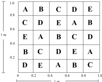
Sampling was made in a systematic scheme in four grids of lags determined using a semivariogram obtained by Gonçalves (1997) for a clay soil. In this way, sampled points were disposed in order to exceed the dependency range limits to ensure the spatial independence among them. The same spacing (20 meters) was used for the sandy soil because the spatial dependency of this soil was not known.
Each equipment was used to take five samples from each sampling point, resulting in 25 samples in an
area of 1 m2. The experimental scheme consisted of Latin
was used to ensure the hypothesis of existing high spatial dependence among them (Figure 1).
Samples were taken at the 20 cm depth with the reference point in the middle of the ring, thus, for the rings used in the instruments A, B, C, D and E the initial depth was 16.5, 18.5, 17.0, 17.5 and 18.5 cm, respectively. A cup sampler with 10 cm of diameter was used to reach the initial depth and the bottom of hole was levelled with an equipment known as “bottom cleaner”, used to turn the base surface soft and remove the free soil, thus avoiding interference in the bulk density measurement.
Sampling was made as follows: first, the five replications with the instruments that do not require trench digging (B50, B100 and SM). After that, the five rings of Kopecky were buried and removed only after sampling with Uhland, which also needs trench digging to take out the rings from the soil.
Immediately after the samples were taken, they were covered with aluminium paper and stocked inside thermal boxes to maintain sample moisture. After levelling the sample corners, the soil was weighted and dried at 105°C for 48 hs and bulk density was determined by the ratio between soil dry weight and the ring volume (EMBRAPA, 1979). Soil porosity was calculated by:
P 1 D
D
s p
= - .100
where P is the soil porosity (%), Ds the soil bulk density
(Mg m-3
) and Dp the soil particle density (Mg m-3
), the last determined by the pycnometer method, described by Blake (1965b).
Statistical analysis was performed using Latin Squares as the experimental scheme as follows: (1) Average, standard deviation and coefficient of variation of soil bulk density data of each instruments were
Figure 1 - Grid of sampled points showing sampling position of each equipment. A=Uhland, B=Kopecky’s Ring, C=Soil Moisture, D=Bravifer AI-50, E=Bravifer AI-100.
C
B
B
B
B
B
E
E
E
E
E
1 m
1 m 0.2
1.0
0.8
0.6
A
A
A
A
A
C
C
C
C
D
D
D
D
0.4D
0 0.2 0.4 0.6 0.8 1.0
calculated for each grid and among the analysed grids for each soil type, and (2) Variance analysis and Tukey’s test for the average values of soil bulk density determined with different instruments, for each grid.
RESULTS AND DISCUSSION
Clayey soil
Average values of soil bulk density, Ds (Mg m-3
), coefficient of variation for each instrument, test F results, minimum significance difference of Tukey’s test and coefficient of variation among the instruments are shown in TABLE 1.
There were significant differences at 1% for grid 1 and 2 and at 5% for grids 3 and 4 for the clayey soil.
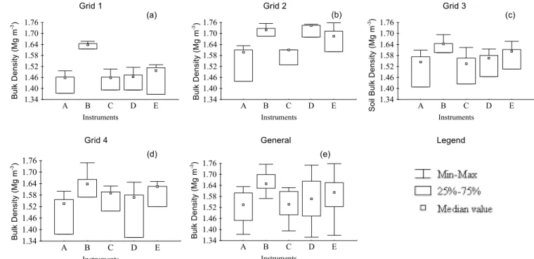
Figure 2 shows the minimum and maximum values of soil bulk density in each grid for the different instruments. Soil bulk density determined by equipment
B in the grid 1 was 0.19 Mg m-3 (13%) higher than the
average values of the other (Figure 2a). In the grid 2, a sample taken with equipment A showed dry and wet weight 10% lower than the other four replications, probably because of the presence of cracks in this
sample which caused a reduction of 0.16 Mg m-3
in relation to the average of the other 4 values. In this grid, samples obtained by this ring were slack inside the ring. Thus, care must be taken to take out the ring from the equipment and in the transport and preparation of sample in the laboratory. This problem may be due to the excessive number of impacts (approximately 40) of the cylinder needed to introduce the rings into the soil or maybe due to roots or other material inside soil samples which reduced their volume after drying (Figure 2b). The minimum values observed for A, C and D instruments in the grid 3 (Figure 2c) and for A and D in the grid 4 (Figure 2d) are associated to the points in which soil sample moisture was higher.
The minimum and maximum values determined by the different instruments in the four sampled grids for the clayey soil are shown in Figure 2e. Equipment B overestimated the soil bulk density, which was 7% (0.105
Mg m-3
) higher than the average of other instruments for this soil.
Sandy soil
Average values of soil bulk density and the coefficient of variation for each equipment in the sampled grids, test F results, minimum significant difference of Tukey’s test and the coefficient of variation among the instruments are shown in TABLE 2.
TABLE 1 - Soil bulk density (Ds) of the clayey soil determined with each equipment, for the 20 cm soil depth. Average values of 5 replications.
Average values followed by the same letter and in the same column do not differ by Tukey’s test at 5%.
Grid1 Grid2 Grid3 Grid4
Equipment Ds CV Ds CV Ds CV Ds CV
Mg m-3 % Mg m-3 % Mg m-3 % Mg m-3 %
A- Uhland 1.44 b 3.6 1.57 c 5.0 1.54 b 5.3 1.52 b 5.7
B- Kopecky's Ring 1.64 a 1.0 1.72 a 1.6 1.64 a 2.4 1.65 a 4.2
C- Soil Moisture 1.44 b 3.3 1.59 bc 2.2 1.54 b 5.0 1.57 ab 3.4
D- Bravifer AI-50 1.46 b 3.3 1.73 a 1.5 1.54 b 5.0 1,55 ab 7.1
E- Bravifer AI-100 1.46 b 5.3 1.69 ab 3.3 1.60 ab 3.5 1.60 ab 3.1
F 15.938 ** 10.394 ** 3.899 * 3.189 *
MSD (5%) 0.096 0.106 0.097 0.126
MSD (1%) 0.124 0.137 0.125 0.163
CV(%) 6.10 5.02 4.46 5.32
Grid1 Grid2 Grid3 Grid4
Equipment Ds CV Ds CV Ds CV Ds CV
Mg m-3 % Mg m-3 % Mg m-3 % Mg m-3 %
A- Uhland 1.71 ab 0.9 1.72 a 1.5 1.78 ab 2.0 1.67 a 3.5
B- Kopecky's Ring 1.77 a 2.9 1.77 a 1.7 1.77 ab 1.2 1.73 a 2.0
C- Soil Moisture 1.67 b 2.6 1.72 a 1.3 1.76 b 1.4 1.68 a 2.7
D- Bravifer AI-50 1.73 ab 2.4 1.74 a 3.1 1.77 ab 1.0 1.70 a 1.6
E- Bravifer AI-100 1.71 ab 2.2 1.74 a 1.8 1.80 a 2.1 1.69 a 1.6
F 7.574 ** 2.822 ** 4.434 * 1.242 n.s.
MSD (5%) 0.056 0.057 0.032 0.088
MSD (1%) 0.072 0.074 0.042 0.114
CV(%) 2.8 2.1 1.6 2.5
TABLE 2 - Soil bulk densities determined with each equipment in the sandy soil for the 20 cm soil depth. Average values of 5 replications.
Average values followed by the same letter and in the same column do not differ by Tukey’s test at 5%.
Figure 3 shows the minimum and maximum values of soil bulk density in each grid for the different instruments. In the grid 1 (Figure 3a), the difference between the lowest value, obtained by the equipment C, and the upper value, obtained by the equipment B, was
14.3% (0.13 Mg m-3). A sample obtained with equipment
D in grid 2 (Figure 3b) presented a value of 1.83 Mg m-3
which is higher than the four other samples (1.72 Mg m-3).
A difference between the lowest value obtained with equipment A and the upper value obtained with D was
0.16 Mg m-3 (9.6%). For grid 4 (Figure 3d), a sample
obtained by equipment A showed a volume reduction of
19.24 cm3 (0.5 cm in the sample height) after drying which
decreased the soil bulk density value (1.57 Mg m-3). This
value was lower than the average value of the four other
replications (1.70 Mg m-3). Difference between the lowest
value obtained with equipment A and the upper value
obtained with B was 0.20 Mg m-3 (12.7%).
The minimum and maximum values determined by the different instruments in the four sampled grids for
the sandy soil are shown in Figure 3e. Equipment B showed the highest average value in all grids, presenting
values 2% (0.045 Mg m-3) higher than the average value
of the other instruments for the sandy soil.
Using the average values of soil bulk density determined with each equipment in the four sampled grids, porosity was calculated for both soils (Figure 4). Samples taken with equipment B presented the highest values of soil bulk density and the lowest values of porosity for both soils, indicating occurrence of soil compaction inside the rings.
Sampling process with equipments A and B needs the trenches digging for removing the soil rings from soil, which makes this process more difficult. Equipment C also needs trench digging, but not necessary for removing the rings, only to introduce it into the soil for depths over 35 cm.
Grid 1 Grid 2 Instruments 1.34 1.40 1.46 1.52 1.58 1.64 1.70 1.76
A B C D E
Bulk Density (Mg m
-3) Instruments 1.34 1.40 1.46 1.52 1.58 1.64 1.70 1.76
A B C D E
Bulk Density (Mg m
-3) Grid 4 Instruments 1.34 1.40 1.46 1.52 1.58 1.64 1.70 1.76
A B C D E
Bulk Density (Mg m
-3) Instruments 1.34 1.40 1.46 1.52 1.58 1.64 1.70 1.76
A B C D E
Soil Bulk Density (Mg m
-3) Instruments 1.34 1.40 1.46 1.52 1.58 1.64 1.70 1.76
A B C D E
Bulk Density (Mg m
-3)
Figure 2 - Minimum and maximum values of soil bulk density for each sampled grid and for the four grids of the clayey soil. A=Uhland, B=Kopecky’s Ring, C=Soil Moisture, D=Bravifer AI-50, E=Bravifer AI-100.
Grid 3
General Legend
Figure 3 - Minimum and maximum values of soil bulk density for each sampled grid and for the four grids of the sandy soil. A=Uhland, B=Kopecky’s Ring, C=Soil Moisture, D=Bravifer AI-50, E=Bravifer AI-100.
Legend Grid 4 Instruments 1.55 1.61 1.67 1.73 1.79 1.85
A B C D E
Bulk Density (Mg m
-3)
Bulk Density (Mg m
-3) Instruments 1.55 1.61 1.67 1.73 1.79 1.85
A B C D E
General Grid 1 Instruments 1.55 1.61 1.67 1.73 1.79 1.85
A B C D E
Bulk Density (Mg m
-3)
Grid 2
Bulk Density (Mg m
-3) Instruments 1.55 1.61 1.67 1.73 1.79 1.85
A B C D E
Grid 3 Instruments 1.55 1.61 1.67 1.73 1.79 1.85
A B C D E
Bulk Density (Mg m
-3)
Figure 4 - Average values of soil porosity calculated from soil bulk density average values. a) clayey soil; b) sandy soil. A=Uhland, B=Kopecky’s Ring, C=Soil Moisture, D=Bravifer AI-50, E=Bravifer AI-100.
34 35 36 37 38 39 40 41 42 43 Po ro si ty ( % )
A B C D E Ge ne ra l
Instrume nts 30 31 32 33 34 35 36 Po ro si ty ( % )
A B C D E Ge neral
Instruments
A B
(a) (b) (c)
(d) (e)
(a) (b) (c)
Received November 25, 1999
CONCLUSIONS
Kopecky’s Ring presented the highest value of soil bulk density for the clayey and sandy soils and overestimated this soil property mainly for the clayey soil. Bravifer AI-50 presented average values closest to the general average value for both soils.
REFERENCES
BLAKE, G.R. Bulk density. In: BLACK, C.A. (Ed.) Methods of soil analysis: Part I. Madison: ASA, 1965a. p.383-390. BLAKE, G.R. Particle density. In: BLACK, C.A. (Ed.) Methods
of soil analysis: Part I. Madison: ASA, 1965b. p.371-373. BUCKMAN, H.O.; BRADY, N.C. Natureza e propriedades dos
solos. Rio de Janeiro: Freitas Barros, 1966. 594p. CONSTANTINI, A. Soil sampling bulk density in the Coastal
Lowlands of South-East Queensland. Australian Journal of Soil Research, v.33, p.11-18, 1993.
DEMOLON, A. Principles d’agronomie: dynamique du sol. Paris: Dunod, 1952. t.1, 522p.
EMPRESA BRASILEIRA DE PESQUISA AGROPECUÁRIA. Manual de métodos de análise de solo. Rio de Janeiro: EMBRAPA, CNPS, 1979. 212p.
FERNANDES, B.; GALLOWAY, H.M.; BRONSON, R.D.; MANNERING, J.V. Efeito de três sistemas de preparo do solo na densidade aparente, na porosidade total e na distribuição dos poros, em dois solos (Typic Argiaquoll e Typic Hapludalf). Revista Brasileira de Ciência do Solo, v.7, p.329-333, 1983.
FOX, W.E.; PAGE-HANIFY, D.S. A method of determining bulk density of soil. Soil Science, v.88, p.168-171, 1959. GOMES, F.P. Curso de estatística experimental. Piracicaba:
Nobel, 1990. 468p.
GOMES, A.S.; PATELLA, J.P.; PAULLETTO, E.A. Efeitos de sistemas e tempo de cultivo sobre a estrutura de um solo podzólico vermelho amarelo. Revista Brasileira de Ciência de Solo, v.2, p.17-21, 1978.
GONÇALVES, A.C.A. Variabilidade espacial de propriedades físicas do solo para fins de manejo da irrigação. Piracicaba, 1997. 118p. Tese (Doutorado) - Escola Superior de Agricultura “Luiz de Queiroz”, Universidade de São Paulo. KIEHL, E.J. Manual de edafologia: relações solo-plantas. São
Paulo: Agronômica Ceres, 1979. 262p.
NESMITH, D.S.; HARGROVE, W.L.; TOLLNER, E.W.; RADCLIFFE, D.E. A comparison of three soil surface moisture and bulk density sampling techniques. Transactions of the ASAE, v.29, p.1297-1299, 1986.
REICHARDT, K.; VIEIRA, S.R.; LIBARDI, P.L. Variabilidade espacial de solos e experimentação de campo. Revista Brasileira de Ciência de Solo, v.10, p.1-6, 1986.
SILVA, A.P.; LIBARDI, P.L.; VIEIRA, S.R. Variabilidade espacial da resistência à penetração de um latossolo vermelho-escuro ao longo de uma transeção. Revista Brasileira de Ciência de Solo, v.13, p.1-5, 1989.
UHLAND, R.E. Physical properties of soils as modified by crops and management. Soil Science Society of America Proceedings, v.14, p.361-366, 1949.