LAND COVER DYNAMICS IN SAVANNA ECOSYSTEM OF BORENA ETHIOPIA

LAND COVER DYNAMICS IN SAVANNA ECOSYSTEM OF BORENA ETHIOPIA

LAND COVER DYNAMICS IN SAVANNA ECOSYSTEM OF

BORENA ETHIOPIA

Thesis

Master of Science in Geospatial Technologies

By

Teshome Abate Beza

Institute for Geoinformatics University of Münster

Main supervisor: Prof. Dr. Edzer Pebesma (University of Münster, Germany) Co-supervisor: Prof. Dr. Pedro Cabral (New University of Lisbon, Portugal) Co-supervisor: Prof. Dr. Pedro Latorre Carmona (University Jaume I Castellon, Spain)

ACKNOWLEDGEMENT

I am very grateful to the European Commission Erasmus Mundus Scholarship program for financing and providing me chance to pursue my studies in the consortium universities. My sincere thanks are also due to coordinators of the program Prof. Dr. Marco Painho, Prof. Dr. Werner Kuhn, Prof. Dr. Joaquín Huerta, and Dr. Chirstoph Brox.

I would like to express my sincere and special thanks to my supervisors Prof. Dr. Edzer Pebesma, Prof. Dr. Pedro Cabral and Prof. Dr. Pedro Latorre for their helpful and valuable comments and suggestion.

I would like to thank Dr.Ayana Angassa for their encouragement and moral support. My thanks and appreciation goes to Mr.Ahmed AbdelHalim M Hassan PhD student in Institute of Landscape Ecology of University of Münster for their assistance during image analysis. I would like to express my thanks to Mr.Getachew Haile for their assistances in provision of all data and GPS facilities.

My deep gratitude also goes to all staff of ISEGI and IFGI for their support and for all its contribution during the program. I would like to thank my classmates and friends Mehash, Paulo, Maia, Chima, Mussie, Dayan, Pearl, Farah, Ermias, and Onyedika other fellow of Erasmus Mundus students and friends for their close friendship and cooperation.

I would like to express my special thanks to my mother, my sisters, my brothers and my friends in Ethiopia for their encouragement. I am not always forgetting the contribution of my father Mr. Abate Beza for my educational life. It is very difficult to make a whole list of individuals who helped me complete this study and it is preferred to express my sincere thanks to all of them.

Last but not the least, deepest and heart-felt gratitude goes to my wife Feiza Ahmed and our son Elias for her encouragement, and moral support.

DECLARATION

I declare that this thesis is my genuine work and that all sources of materials used for this thesis have been duly acknowledged. I solemnly declare that this thesis is not submitted to any other institution anywhere for the award of any academic degree, diploma, or certificate.

Teshome Abate Beza

Muenster, Germany

Land cover dynamics in savanna ecosystem of Borena Ethiopia

ABSTRACT

KEYWORDS

Land use change

Landscape structure

Spatial metrics

Vegetation cover

Borena pastoralist

ACRONYMS

ETM+ Enhanced Thematic Mapper plus

FAO World Food and Agriculture Organization GIS Geographical Information System

GLCF Global Land Cover Facility GPS Global Positioning System

IHDP International Human Dimensions Programme IGBP International Geosphere-Biosphere Programme ILRI International Livestock Research Institute LPI Largest Patch Index

LUCC Land Use and Land Cover Change MSS Multispectral Scanner

NMA National Metrological Agency

NDVI Normalized Difference Vegetation Index SHDI Shannon’s Diversity Index

SHEI Shannon’s Evenness Index TM Enhanced Thematic Mapper

INDEX OF THE TEXT

ACKNOWLEDGEMENT ... ii

ABSTRACT ... iv

KEYWORDS ... v

ACRONYMS ... vi

INDEX OF THE TEXT ... vii

INDEX OF TABLES ... ix

INDEX OF FIGURES ... x

LISTS OF ANNEXE TABLES ... xii

LISTS OF ANNEXE FIGURES ... xii

1. INTRODUCTION ... 1

1.1 Study background ... 1

1.2 Statement of problem ... 2

1.3 Aim and objectives ... 4

1.4 Research hypothesis and question ... 4

1.5 Thesis structure ... 5

1.6 Tools used in the study ... 5

1.7 Significance of the study ... 6

2 LITERATURE REVIEW ... 7

2.2 Remote sensing and land use and land cover change studies ... 9

2.3 Change detection techniques ... 11

2.4 Satellite image classification methods... 13

2.5 Landscape metrics and land use and land cover change studies ... 14

2.6 Land use and land cover change in Ethiopia ... 15

3 DESCRIPTIONS OF STUDY AREA AND DATA ... 18

3.1 Description of study area ... 18

3.2 Climate and land use ... 19

3.3 Topography and vegetation ... 21

3.4 Data type ... 21

3.4.1 Reference data... 23

4 METHODOLOGY ... 24

5 RESULT AND DISCUSSION ... 32

5.1 Result ... 32

5.1.1 Classification accuracy assessment ... 32

5.1.2 Land use and land cover classification 1987-2003 ... 35

5.1.3 Change detection analysis ... 41

5.1.4 Change detection using NDVI ... 50

5.1.5 Spatial patterns of land use and land cover dynamics ... 55

5.2. Discussion ... 61

6. CONCLUSION AND RECOMMENDATION ... 68

BIBLIOGRAPHY ... 70

INDEX OF TABLES

Pag.

Table 1 Mean monthly rainfall in mm (1980-2004) and the coefficient of variation, ... 20

Table 2 Description of Landsat image data used in the study ... 22

Table 3 Image spectral bands of Landsat TM and ETM and their importance ... 23

Table 4 Land use and land cover class nomenclature used in the study area ... 28

Table 5 Class and landscape metrics adopted and used in this study ... 31

Table 6 Landsat TM classification accuracy for 1987 ... 34

Table 7 Landsat TM classification accuracy for 1995 ... 34

Table 8 Landsat TM classification accuracy for 2003 ... 35

Table 9 Area statistics and percentage of the land use/cover units in 1987-2003 ... 36

Table 10 Overall amount, extent and rate of land cover change (1987-2003) ... 41

Table 11 Land-use/cover transition matrix showing major change in the landscape ... 43

Table 12 Land-use/cover transition matrix showing major changes in the landscape (Km2), Yabelo, ... 46

Table 13 Land-use/cover transition matrix showing major changes in the landscape ... 48

Table 14 Area of vegetation (%) change calculated by difference of NDVI ... 53

Table 15 The calculated landscape metrics at the landscape level ... 57

INDEX OF FIGURES

Pag.

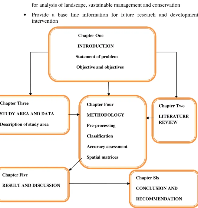
Figure 1 The flow diagram of thesis outline ... 6

Figure 2 Map of study area, Yabelo ... 18

Figure 3 Mean annual rainfall (mm) of Yabelo district from 1980 to 2004, Borana ... 19

Figure 4 Mean annual minimum and maximum Temperature of Yabelo district.... 20

Figure 5 The flow chart for image processing and LUCC change detection and landscape metrics ... 26

Figure 6 RGB composite Landsat images used for classification ... 27

Figure 7 Land use land cover classification map for 1987 ... 37

Figure 8. Land use land cover classification map for 1995 ... 38

Figure 9 Land use land cover classification map for 2003 ... 39

Figure 10 Nature of relative land cover changes 1987 to 2003 ... 41

Figure 11.Contribution in net land use change experienced in each land use type (% area), 1987- 2003. ... 45

Figure 12 Contribution in net land use change experienced in each land use type (% area), 1987-1995 ... 47

Figure 13 Contribution in net land use change experienced in each land use type (% area), ... 49

Figure 15 NDVI of 1987 ... 51

Figure 16 NDVI of 1995 ... 52

Figure 17 NDVI of 2003 ... 52

LISTS OF ANNEXE TABLES

Pag.

Table 1 Mean monthly rainfall of Yabello district from 1980 to 2004,

Borana rangelands, Ethiopia ... 77

Table 2 Mean monthly maximum Temperature of Yabello district from 1980 to

2004,Borena rangelands, Ethiopia ... 78

Table 3 Mean monthly minimum Temperature of Yabello district from 1980 to

2004,Borana rangelands, Ethiopia ... 79

Table 4 Contribution to net land use change by each land cover (%) of area

(1987-2003) ... 80

LISTS OF ANNEXE FIGURES

Pag.

1. INTRODUCTION 1.1 Study background

Land use and land cover change (LUCC) information constitutes key environmental information for many scientific, resource management, policy related issue, as well as for a range of human activities. As a result, LUCC have become a major focus for the International Geosphere-Biosphere Programme (IGBP) and the International Human Dimensions Programme (IHDP) at different scale. Since the 1970s, concerns about changes in LUCC have emerged in the research on global environmental change (Lambin et al., 2003) due to LUCC change are closely linked to the sustainability of socio-economic development and livelihood of people (Lambin et al., 1997).There is complex and dynamic LUCC change at various scales, which have global environmental implication. Thus due to the dynamic nature of LUCC change the scope of problem still remains an area of active study and debate. Hence, detailed and continuous study at different scale is needed (Fuller and Chowdhury, 2006). Adequate and accurate information in LUCC cover change is a key to many diverse applications for instance, information on LUCC change is required to understand and manage the environment at variety of spatial and temporal scales. It is essential for monitoring global change and for sustainable management of natural resource. It is also input data for a range of environmental models and policy-driven need (Rosenqvist et al., 2003).

cover change in many arid savanna ecosystem of Ethiopia is scanty. Thus, assessing of LUCC change dynamic, driving force and its impact behind LUCC change is essential. To these end timely and accurate change detection of Earth's surface features is extremely important for understanding relationship and interaction between human and natural phenomena in order to promote better decision making (Lu et al., 2004).

Recently, a substantial amount of data from the Earth’s surface is collected using Geospatial technologies such as Global Position System (GPS), Geographical Information System (GIS) and Remote Sensing. Remote Sensing and GIS provide an excellent source of data over large geographical area from which updated LUCC information and change can be extracted, analyzed and predicated efficiently. Many studies have demonstrated remote sensing using satellite image detect and monitor LUCC change in savanna ecosystem (Duadze, 2004; Bedru, 2006). Research proves that remote sensing can be considered a useful tool for studying arid and semi-arid ecosystem.

1.2 Statement of problem

Rangelands in Ethiopia are located below an elevation of 1 500 masl. They cover about 61-65% of the total area of the country and are characterized by arid and semi-arid agro-ecologies, experiencing a relatively harsh climate with low, unreliable and erratic rainfall. The rangelands are home to 12-15% of the human population and 26% of the total livestock population and provide habitat for many wildlife species. Pastoralism and agro-pastoralism are the dominant type of land use system in these areas. Livestock in the rangeland play a significant role in the national economy. However, many of these rangelands at present are degrading owing to natural and human-induced factors (Abule et al., 2005).

finest savanna grazing land in East Africa and had good ecological potential for livestock production (Hogg, 1997). However, many studies (Coppock 1994; Gemedo Dale, 2004; Homann, 2004; Solomon et al., 2006; Angassa and Oba, 2008) reported recently the condition of Borena rangeland has been degraded and transformed due to climate and human induced factors including land degradation, expansion of bush cover, expansion of cultivation of crop, frequent and recurrent drought, ban on use of fire, human population pressure and weakening of traditional indigenous management system. Such pastoral land use transformation are affecting the sustainable use of savanna landscape as well as pastoral production system (Angassa and Oba, 2008).These pastoral land use transformation has occurred at different degree of magnitude and temporal scale. Several studies have reported land cover change in Borana rangeland currently has accelerating and causing wide range environmental problem (e.g. rangeland degradation and bush encroachment).Proper understanding of land use transformation scenario and quantifying the extent and rate of change is critically important owing to the changing patterns of land cover reflect changing environment, economic and social conditions of the area.

change of savanna landscape covering period of 1980’ 1990’, and 2000’. These periods are selected because of dramatic change, which have been observed in range development and consequently change in traditional land use and vegetation shift in southern Ethiopia over the last 4-5 decade.

1.3 Aim and objectives

The overall objective of the study was to analysis LUCC change pattern using multi-temporal Landsat imageries in three different time series (1987, 1995 and 2003). Furthermore, it has designed to studies landscape structure in different temporal and spatial scale.

Specific objectives:

• To map and determine the extent and rate of LUCC change using post and

pre classification approaches

• To analyze spatial pattern and landscape structural change using selected

spatial metrics.

• To generate some baseline information for future research and development

activities

1.4 Research hypothesis and question Hypothesis

We hypothesized that whether significant variation in LUCC dynamic and landscape structure change has observed in the rangeland of Borena in given spatio-temporal scale.

Research question

In order to meet the hypothesis and objectives, the study set the following research questions

• Is there any land use/land cover change in the study area?

• What was the spatial extent of the land cover change and where was the

• Is there any landscape structural change in the study area?

• Is remote sensing a suitable tool for detection of LUCC change in the arid

and semi arid environment?

• Is NDVI a suitable tool for detection of vegetation change in the arid and

semi arid environment?

1.5 Thesis structure

The thesis has organized into six main chapter outlined and presented in Figure1. The first chapter deals with the introduction and statement of the problem, objectives, hypothesis and research question. The second chapter covers review of related literature which include definition and concept of LUCC change, remote sensing and LUCC change, different change detection technique, image classification method, landscape metrics and LUCC change in Ethiopia. The third chapter described about the study area and type and nature of data set used. In this chapter location, climate, topography, vegetation and the main land use practice was discussed. Chapter four emphasizing mainly on research methodologies which include image pre-processing, classification, accuracy assessment, change detection and spatial metrics analysis procedure. Chapter five deals on result and discussion. Finally, chapter six covers conclusion and recommendation and limitation of the study.

1.6 Tools used in the study

1.7 Significance of the study

Land use and land cover change studies are important tool for land manager and decision makers in formulating appropriate land use policy as well as locating development program for sustainable use of savanna ecosystem in southern Ethiopia. The result of this study would provide information relevant to contribute in the rangeland management plan. It is also expected to:

• Provide information on the status and dynamic of LUCC change of area and

also provide information the use of remote sensing from satellite imagery for analysis of landscape, sustainable management and conservation

• Provide a base line information for future research and development

intervention

Figure 1 The flow diagram of thesis outline

Chapter One

INTRODUCTION

Statement of problem

Objective and objectives

Chapter Three

STUDY AREA AND DATA

Description of study area

Chapter Two

LITERATURE REVIEW

Chapter Five

RESULT AND DISCUSSION

Chapter Four

METHODOLOGY

Pre-processing

Classification

Accuracy assessment

Spatial matrices

Chapter Six

CONCLUSION AND

2 LITERATURE REVIEW

This chapter highlight literature review related to LUCC change done so far at various scale and the review mainly focus on the definition and concept of LUCC change, remote sensing and LUCC change, change detection techniques, image classification method, landscape metrics and LUCC change and LUCC change in Ethiopia. These topics have reviewed under the following sub-topic.

2.1 Definition and concept of land use and land cover change

Land use and land cover change is a general term for the human modification of Earth's terrestrial surface. Though humans have been modifying land to obtain food and other essential for thousands of years, current rate, extent and intensities of LUCC change are far greater than ever in history, driving unprecedented change in ecosystem and environmental process at local, regional and global scale. These changes encompass the greatest environmental concern of human population today including climate change, biodiversity loss and the pollution of water, soil and air. Monitoring and mediating the negative consequence of LLCC change has therefore become a major priority of researcher and policymaker around the world. (http://www.eoearth.org/article/Land-use_and_land-cover_change1).

Before discussing about LUCC change, it is important to define the term. In order to appreciate the definition and concept of land use and land cover, it may be necessary to, first of all, define the term “land”. Land is a complex and dynamic combination of factors: geology, topography, hydrology, soils, microclimates, and communities of plant and animal that are continually interacting under the influence of climate and people activities (FAO, 1998) it is the basic natural resource, which provide space, energy and nutrients that are essential for all biochemical metabolisms occurring in any organism. Land plays a key role in major biogeochemical cycle both within ecosystem and globally (FAO, 1998). Generally, land can be considered in two domains: (1) land in its natural condition and (2) land

1

that has been modified by human being to suit a particular use or range of use. The natural capability of land to meet a certain anthropogenic activity in a broad sense is referred to as land quality, and this is traditionally interpreted in terms of land resource, which determines land use. Historically, land has been exploited in different ways, from a simple watching of landscape and primitive collection of herbs to artificially generated industrial areas (Stolbovoi, 2002). In these ways, humans are adapting to land capacity or rebuilding land to fit their demand. Many authors or groups have defined “land use” and “land cover. Land cover it refers to the physical and biological cover of the earth's surface including artificial surfaces, agricultural areas, forests, (semi-)natural areas, wetlands, water bodies. Whereas, land use is a more complicated term, natural scientists define land use change is the conversion of land use due to human intervention for various purpose, such as for agriculture, settlement, transportation, commercial, recreation, mining and fishery (Turner et al., 1993). While social scientists and land managers define land use more broadly to include the social and economic purpose and context for and within which lands are managed (or left unmanaged), (e.g. as subsistence versus commercial agriculture ,rented vs. owned, or private vs. public land (http://www.eoearth.org/article/Land-use_and_land-cover_change).Thus land use encompasses a wide range of natural and socio-economic aspects and their interrelations (Stolbovoi, 2002).

biophysical and socio-economic factors which may occur at various temporal and spatial scale. The driving force to this change could be environmental, economic, land policy and development program, technological, demographic, and or other factors.

2.2 Remote sensing and land use and land cover change studies

Remote Sensing is the science and art of obtaining information about an object, area, or phenomenon through the analysis of data acquired by a device that is not in contact with object, area, or phenomenon under investigation (Lillesand and Kiefer, 1994). The modern usage of the term remote sensing has more to do with the technical ways of collecting airborne and space borne information. Earth observation from airborne platforms has a one hundred and fifty years old history although the majority of the innovation and development has taken place in the past thirty years. The first Earth observation using a balloon in the 1860s is regarded as an important benchmark in the history of remote sensing. Since then platforms have evolved to space stations, sensors have evolved from cameras to sophisticated scanning device and the user base has grown from specialized cartographers to all rounded disciplines. It was the launch of the first civilian remote sensing satellite in the late July 1972 that paved the way for the modern remote sensing applications in many fields including natural resources management (Lillesand et al. 2004). For the past couple of decade the application of remote sensing not only revolutionized the way data has been collected but also significantly improved the quality and accessibility of important spatial information for natural resources management as well as LUCC change studies.

the satellite type. The major ones whose data are most commonly used for the study of the Earth’s resources including Landsat the Multispectral Scanner (MSS, 79m resolution), Landsat Thematic Mapper (TM, 30m resolution) and Landsat Enhance Thematic Mapper (TM, 30m resolution) has medium resolution sensors which are suitable for the study of land use and land cover, and have been used to derive detailed land use classification of many part of the world including the tropics (Purevdor et al., 1998). Major change to the surface of the earth such as desertification, deforestation, and other natural and anthropogenic events can be detected, examined, measured and analyzed using Landsat data. The information obtainable from historical as well as current Landsat data plays key roles in the study of surface change through time (ERDAS, 1999).

2.3 Change detection techniques

Change detection is the process of identifying differences in the state of an object or phenomenon by observing it at different times (Singh, 1989). Thus, change detection is an important process in monitoring and managing natural resource and understanding the nature of change in the use of land resources. Change detection determines change of a particular object between two or more time periods to produce a quantitative spatial analysis in an area of interest (Macleod and Congalton, 1998). The four aspects of change detection which are important when monitoring natural resources and land use cover are detecting the change that have occurred, identifying the nature of the change, measuring the area extent of the change and assessing the spatial pattern of the change (Singh, 1989; Macleod and Congation,1998). However, the accuracy of change detection depend on many factors, including, precise geometric registration between multi-temporal images, calibration or normalization between multi-temporal images, availability of quality ground reference data, the complexity of landscape and environment of the study area, using appropriate change detection algorithms and others. Thus, identifying a suitable change detection technique has significance contribution to produce good change detection result. The temporal, spatial, spectral and radiometric resolutions of remotely sensed data have also a significant impact on the success of remote sensing change detection. In general, when selecting remote sensing data for change detection applications, it is important to use the same sensor, same radiometric and spatial resolution data with anniversary or very near anniversary acquisition dates in order to eliminate the effects of external sources such as sun angle, seasonal and phonological differences.

spectral change detection or post-classification methods (Singh 1989). Post classification change detection, two multi-temporal images are classified separately and labeled with proper attributes. The area of change is then extracted through then direct comparison after obtaining the classification result. With the post-classification procedure basic issues are the accuracies of the component classification and more subtle issues associated with the sensors and data preprocessing method (Lu and Weng 2007). In pre classification spectral change detection where changes occur in the amount or concentration of some attribute that can be continuously measured (Coppin and Bauer, 1994). In spectral change detection, image of two dates are transformed into a new single-band or multi-band image, which contains the spectral changes. The resultant image must be further processed to assign the changes to specific land cover types. Since these methods are based on pixel-wise or scene-wise operations, they are sensitive to image preprocessing such as registration and co-registration accuracy. Discrimination of change and no-change pixels is of the greatest importance in successful performance of these methods. A common method for discrimination is use of statistical threshold. In this method a careful decision is required to place threshold boundaries to separate the area of change from no-change (Singh, 1989).

Vegetation Index, and Transformed Vegetation Index. In this study Normalized Vegetation Index is used to observe the general greenest of the study area.

2.4 Satellite image classification methods

Satellite image classification is the process of assigning classes to the pixels in images. It is a complex and time consuming process, and the result of classification may be influenced by various factors such as nature of input images, classification method, scale of the study area, and post classification processing. In general, image classification method can be grouped as supervised and unsupervised, or parametric and nonparametric, or hard and soft (fuzzy) classification, or per-pixel, sub pixel, and per field (Lu and Weng 2007). Among all classification method some of them will be discussed. Pixel-based classification, in this method, each pixel is classified based on the spatial arrangement of edge features in its local neighborhoods (Im et al. 2008). Image classification at pixel level could be supervised or unsupervised; parametric and hard classifiers. In a supervised classification method the image analyst has responsible for the supervises the pixel categorization process by specifying to the algorithm, class definitions, or signatures of the various land use and land cover types present in a scene to train the algorithm (Lillesand and Kiefer, 1994). Maximum likelihood of supervised classifier is the most commonly used method.

objects, instead of individual pixels (Lu and Weng, 2007).The eCognition method is so far the most commonly used object-oriented classification (Lu, 2004). The other classification approach is advanced classification approaches. In recent year various advanced image classification approaches have been widely developed and applied such as artificial neural networks, expert systems, fuzzy-set theory, decision tree classifier, etc. ( Lu and Weng, 2007)

2.5 Landscape metrics and land use and land cover change studies

Knowing the landscape structure, the nature and magnitude of its change, and how it affects landscape processes are essential in the sound management of land and their resource. Particular, important for resource manager because its need spatial and temporal information to make decision about landscape patch size, the dispersal or aggregation of activities, edge densities, and connectivity in the landscape (McGarigal, et al., 2002). Landscape is defined as a heterogeneous land area composed of a cluster of interacting ecosystems that is repeated in similar form throughout (Forman and Godron, 1986). It is composed typically of various types of landscape elements (patches). Patches represent relatively discrete area (spatial) of relatively homogeneous environmental condition. Landscape metrics is one of imperative method for understanding the structure, function and dynamic of landscape. The ability to quantify landscape structure is fundamental to the study of landscape function and change (McGarigal and Marks, 1994).

contagion, and interspersion, dispersion. In many field of research including land use and land cover change, landscape metrics are used to quantify the spatial heterogeneity at different level (patch, class and landscape). Metrics at patch level measure and characterize the spatial character and context of patch, parameter including the size and shape of each individual patch. Whereas class metrics measure, the characteristic of a particular class (e.g. the number of patch for each class, the percentage of the landscape occupied by that class etc). Metrics at the landscape level measure for over all patch type or classes over the entire landscape. Landscape metrics can be used as indicators for watershed integrity, landscape stability, resilience, biotic integrity and diversity (McGarigal, et al., 2002). In Europe, the Joint Research Centre of the European community has suggested metrics based approaches utilizing remotely sensed image used to develop biodiversity indicators at the landscape level (JRC, 1999).Many literatures indicated that so far varieties of landscape metrics have been developed. However, the most commonly used metrics include area, patch density, patch size and variability, edge, shape, nearest-neighbour, and diversity metrics (McGarigal and Marks,1994). In this study different metrics to characterize the savanna landscape composition and spatial configuration at different spatial and temporal was used

2.6 Land use and land cover change in Ethiopia

2007), rift valley area (Rembold et al., 2000) are the major change observed over the last 4-5 decade. Shibru et al. (2003) reported the effect of LUCC in causing major gullies and quantified the rate expansion and their effect on the livelihood of people in eastern and central highland of Ethiopia. Similarly many studies reported there was depletion of natural vegetation and reduction of habitat structure over the past 4-5 decade. For example FAO, 2001 estimate the annual rate of deforestation in Ethiopia in the range of 36,600 to 40,000 hectare.

in one of the his study sites, while the other lost all of its original 54% woodland cover.

3 DESCRIPTIONS OF STUDY AREA AND DATA 3.1 Description of study area

The study was conducted in Borana rangeland, Southern Oromiya, Yabelo. The Borana rangelands are located in the southern part of the Ethiopian lowland and it covers a total land of 95,000km².Yabelo district is found in central Borana rangeland of south Ethiopia (Coppock, 1994) and the district is situated 570 km south of Addis Ababa (capital town of Ethiopia) and it covers an area of about 5523km².The district is borders Hagere Mariam in North, Arerro in East, Dire in south and Teltele district in West respectively. The areas are predominantly occupied by pastoral people, whose livelihood is mainly dependent on extensive livestock production; mainly keep cattle (232,949) along with goat (99,681), sheep (39,043) and camel (22,972). The Booran are the dominant pastoralist ethic group, this group had well established and organized indigenous system on water technology, grazing land management for example, Borana pastoralist classify their grazing land both spatially and temporally. Furthermore they had a highly organized and durable social organization of the gada system.

3.2 Climate and land use

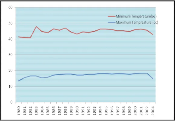
The climate of the area is categorized under arid and semi arid agro ecology. Rainfall data obtained from National Metrological Agency (NMA) (1980 to 2004) indicated that in Yabelo mean monthly rainfall ranged from 9.17mm to142.1mm (Figure 3 and Table1). The average annual rainfalls varied and mean annual rainfall (526.75mm). Rainfall is bimodal with 60% of the annual rainfall occurring between March and May (main rainy-season) followed by a minor peak between September and November (small rainy-season). Mean annual temperature of the area varied from 19°C to 24°C. However, the mean maximum and minimum temperature is 27.74°c and 16.45°c, respectively (Figure 4 and Table 1). A drought is common in the area and has occurring frequently some of the drought occurred years in the study area were 1975/1976, 1979/1980, 1984/1985, 1987/1988, 1991/1992, 1995/1996, 1999/2000 (Sabine et al., 2005). Out of the total land area, 10% is arable, 60%rangelands, 10% forest, and the remaining 20% is considered degraded or otherwise unusable.

Figure 3 Mean annual rainfall (mm) of Yabelo district from 1980 to 2004, Borana

Figure 4 Mean annual minimum and maximum Temperature of Yabelo district from 1980 to 2004, Borana rangelands, Ethiopia (sources:NMA)

Table 1 Mean monthly rainfall in mm (1980-2004) and the coefficient of variation, maximum and minimum temperature in Yabelo, Ethiopia

Month J F M A MA J JUL AU SEP O N D

RF 12.91 21.19 43.79 148.09 86.77 17.40 18.24 9.43 13.87 58.15 74.80 33.96

Max Tep 31.41 32.05 31.14 27.82 26.31 24.83 24.48 25.65 26.29 26.41 27.37 29.02

MinTep 19.06 17.81 18.48 17.57 16.97 16.19 15.69 15.44 16.19 16.93 17.57 16.30

RF CV 176 98 97.95 79.53 99.51 124.1 325.5 88.11 141.7 83.65 78.01 108.9

3.3 Topography and vegetation

The topography is consists of isolated mountains, valleys and depression, and an altitude range of 1000 to 1,700 m.a.s.l. The Borana plateau is dominated by savanna type of vegetation containing a mixture of perennial herbaceous and woody plant (Coppock, 1994).These savanna communities are varying from grassland to bush encroached area. The variation in woody and herbaceous materials as well as marked shifts in composition that occurred in response to grazing, browsing, burning and droughts or various combination of these. According to Haugen (1992) woodland of Yabelo rangelands are characterized by species from the genera Combretum and Terminalia, whereas the bush land and thicket, which cover major parts of the Borana lowlands, are dominated by Acacia and Commiphora species. Besides, species of the genera Boscia, Maerua, Lannea, Balanites, Boswellia and Aloe are common in the study area. The dominant herbaceous plants were perennial grasses. The Borana rangeland is a water-limited environment with the major source of water for both human and livestock were wells and ponds. The soils of the study area are predominated with sandy-loam textural classes. The black clay soil (Vertisols) cover nearly 30% of the area and other types of silty soil occupied the balance. The valley and bottomlands are occupied by cracking and volcanic light colored soils having slight drainage impedance, relatively high fertility and high water holding capacity (Coppock, 1994).

3.4 Data type

Table 2 Description of Landsat image data used in the study Reference

year

Sensor Resolution WRS path/raw

Date of acquisition

1987 Landsat TM 30m 168/057 Feb,09,1987

1987 Landsat TM 30m 168/056 Feb,09,1987

1995 Landsat TM 30m 168/057 Jan,30,1995

1995 Landsat TM 30m 168/056 Jan,30,1995

2003 Landsat ETM+ 30m 168/057 Jan,12,2003

2003 Landsat ETM+ 30m 168/057 Jan,12,2003

For change detection analysis, it is important to acquire imagery of anniversary dates and similar season to minimize variation in reflectance of a feature caused by season and sun-angle differences (Coppin et al. 2004). Even though selection of appropriate imagery is an important component for successful LUCC change analysis, data selection was primarily determined by availability of imagery covering the study area. The TM and ETM+ imagery used in this study were cloud free and acquired for month of January to February which is dry season image.

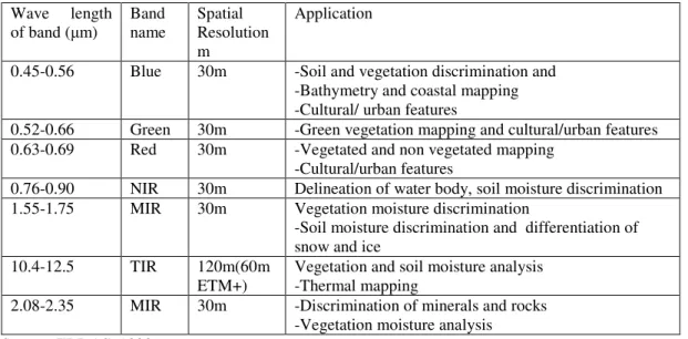
Table 3 Image spectral bands of Landsat TM and ETM and their importance

Wave length

of band ( m) Band name Spatial Resolution m

Application

0.45-0.56 Blue 30m -Soil and vegetation discrimination and -Bathymetry and coastal mapping -Cultural/ urban features

0.52-0.66 Green 30m -Green vegetation mapping and cultural/urban features 0.63-0.69 Red 30m -Vegetated and non vegetated mapping

-Cultural/urban features

0.76-0.90 NIR 30m Delineation of water body, soil moisture discrimination 1.55-1.75 MIR 30m Vegetation moisture discrimination

-Soil moisture discrimination and differentiation of snow and ice

10.4-12.5 TIR 120m(60m ETM+)

Vegetation and soil moisture analysis -Thermal mapping

2.08-2.35 MIR 30m -Discrimination of minerals and rocks -Vegetation moisture analysis Source: ERDAS, 1999

3.4.1 Reference data

It is necessary to use different reference data sets to develop training samples, classification and accuracy assessment. It is true that ancillary data such as high resolution imageries and existing map of the study area was essential for classifying and assessing the accuracy of the classification. In relation to this study, land use map of study area, road network, district boundary, protected area map, Google earth map and other meteorological data were used as ancillary data for classification, accuracy assessment and LUCC change analysis. The land use map, road network were acquired from International Livestock Research Institute (ILRI) (http://64.95.130.4/gis/search.asp2) and Biomass Inventory Planning Project. Furthermore, topographic map at the scale of 1:50000 which cover the entire study area was obtained from the Ethiopian Mapping Agency. In addition, over 442 GPS point ground truth data were gathered from study area and used as accuracy assessment.

2

4 METHODOLOGY

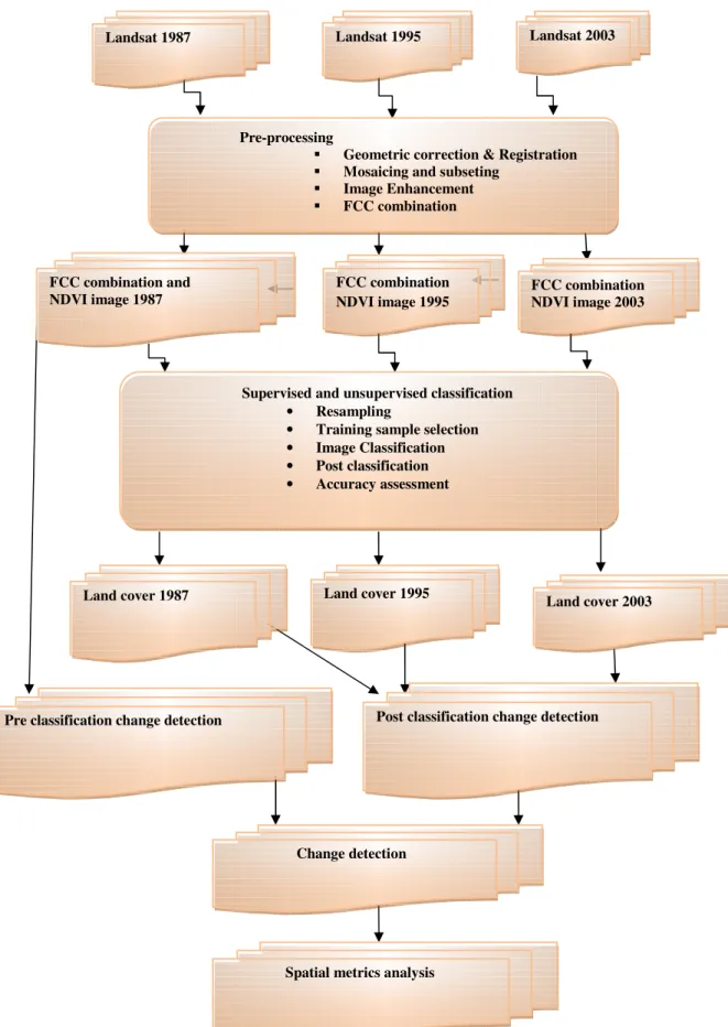
Imageries and ancillary data were processed to determine the LUCC change, pre- and post-classification method was used to detect change in land use and land cover class. The flow chart of the procedure for image pre processing, enhancement, classification, accuracy assessment, and spatial metrics analysis was depicted in Figure 5. Data from remotely sensed image obtained from different sources are not usually ready to use directly, because of satellite data obtained from various sensors undergo some degree of geometric and radiometric distortion due to earth rotation, platform instability, atmospheric effect, etc. Thus need to a series of preprocessing steps to remove errors associated with acquisition of multi-temporal data and to correct the error during scanning, transmission and recording of the data. The preprocessing steps used are geometric correction, image registration (georeferencing); mosaicking, and subsetting unnecessary features, edge maching (ERDAS, 1999).

Image registration and Geometric correction; Image registration is the process of transforming the different set of data into one coordinate system. All the Landsat TM and ETM+ images had been already orthorectified by the image supplier to Universal Transverse Mercator (UTM) projection on the WGS84 datum, UTM Zone 37. For further analysis image to image registration were done using IDRIS ANDES and edge matching also done taking 1987 image as reference image using AUTOSYNC tools of Erdias imagine soft ware.

the boundary of the study area was used to mask the image and cut the area of interest from all satellite imagery

Image Enhancement; Image enhancement deals with the procedures of making a raw image more interpretable for a particular application. There are a number of method can be used to undertake enhancement of image. In this study, simple contrast, haze reduction, linear stretching, and histogram matching were used.

Radiometric correction; Radiometric correction can be achieved through many methods such as detailed correction of atmospheric effect, calibration to surface reflectance, and bulk correction of atmospheric effect (dark object subtraction). Detailed correction of atmospheric effect requires detailed atmospheric information such as humidity and temperature at time of image acquisition, which is not easily available. Calibration to surface reflectance requires a spectral library of the darkest and brightest object in the image. Unfortunately no spectral library and no field spectrometer data have been available. In this study, radiometric correction such as linear stretching, haze reduction, histogram matching was done.

Figure 5 The flow chart for image processing and LUCC change detection and landscape metrics Analysis

Landsat 1987 Landsat 1995 Landsat 2003

Pre-processing

Geometric correction & Registration Mosaicing and subseting

Image Enhancement FCC combination

FCC combination and NDVI image 1987

FCC combination NDVI image 1995

FCC combination NDVI image 2003

Supervised and unsupervised classification

• Resampling

• Training sample selection

• Image Classification • Post classification

• Accuracy assessment

Land cover 1987 Land cover 1995

Land cover 2003

Post classification change detection

Change detection

Band Selection for FCC (false color composite): After tested different band combination, RGB 4, 3 and 2 was selected for 1987 TM and 2003 ETM+ and RGB 7, 4 and 2 was used for TM 1995. It has been found that standard RGB 4, 3 and 2 band combinations provide very useful information for land use mapping. Similarly, a false color composite of RGB 7, 4 and 2 is particularly suitable for provide useful information for arid and desert region (Figure 6)

1987FCC432 1995FCC742 2003FCC432

Figure 6 RGB composite Landsat images used for classification

Normalized Difference Vegetation Index: Normalized Difference Vegetation Index (NDVI) is a data transformation which reduces data dimensionality. NDVI is the most widely used of all vegetation indices because it requires data from only the red and near-infrared portion of the electromagnetic spectrum, and it can be applied to virtually all remotely sense multi-spectral data types. In this study NDVI was computed to quantify the general vegetation condition such as relative greenness and change detection (ERDAS, 1999). The NDVI is defined as reflectance in the near-infrared (NIR) range minus reflectance in the visible red (R) spectrum portion divided by their sum. It is expressed mathematically as follows

NDVI= (NIR - R)/ (NIR+ R)

of their relatively high reflectance in NIR and low reflectance in the visible wavelengths. On the contrary, water and bare soil will have higher reflectance in visible wavelength than in the NIR, thus these features yield negative and near-zero values (ERDAS, 1999). NDVI is not always suitable especially in semi-arid area where the vegetation cover is very sparse and soil background in reflectance value is very high (mixed pixels).Vegetation indices are likely to underestimate live biomass in desert, they are insensitive to nonphotosynthetic vegetation and are sensitive to soil color (Okin and Roberts, 2004).

Land class nomenclature: The land cover classes used in this study was adopted from the classification scheme used by the Ministry of Agriculture of Ethiopia and based on classification criteria for East African rangeland (Pratt and Gwynne, 1977) and based on the previous studies made in the similar study area (Diress et al, 2010, Getachew et al., 2010). For the sake of simplicity, land class nomenclature was modified into seven classes and summarized in Table 4.

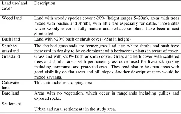
Table 4 Land use and land cover class nomenclature used in the study area

Land use/land

cover Description

Wood land Land with woody species cover >20% (height ranges 5–20m), areas with trees mixed with bushes and shrubs, with little use especially for cattle. Those sites where woody cover is fully mature and herbaceous plants have been almost eliminated.

Bush land Land with >20% bush or shrub cover (<5m in height) Shrubby

grassland

The shrubed grasslands are former grassland sites where shrubs and bush have increased in density to be co-dominant with herbaceous plants in terms of cover Grassland Grassland with <20% bush or shrub cover, Grass and herb cover with scattered

trees and shrubs, areas with permanent grass cover used for livestock grazing including communal and protected areas. They tend also to be open areas with good visibility on flat areas and hill slopes Another descriptive term would be mixed savanna.

Cultivated

land This unit includes cropping area

Bare land Areas with no vegetation, which occur in rangelands including gullies and exposed rocks.

Settlement

Image Classification

After the necessary image preprocessing, classification was computed. The classification of image was done using both unsupervised and supervised classification. Initially, unsupervised classification was used to get insight about the overall class and to identify the training site. The result of unsupervised classification was used as a guide for the selection of training site for supervised classification and it also gives preliminary information on the potential spectral clusters to be assigned to thematic classes. Finally, image was classified at pixel level using supervised classification of maximum likelihood classifier approaches. Seven land cover classes were identified, namely wood land, bush land, grassland, shrubby grassland, bare land, cultivation and settlement.

Post-classification enhancement: Post-classification enhancement such as filtering of the final classification result using different filter techniques to reduce the heterogeneity of the classified image is essential. However, filtering was not carried out in this study because it tended to generalize the classification to the extent that some mapping units, e.g., cultivation area and settlements totally disappeared. Duadaze (2004) and Su (2000) made a similar observation. Finally, maps were prepared using the ARC GIS 9.3 version. A post and pre classification comparison method was used for detecting of land use and land cover change where Landsat image for each year was classified and labeled independently and then comparison were made for the generated LUCC maps of 1987–1995, 1995–2003 and 1987-2003 the area of change also determined and compared.

Accuracy assessment

number of sample units assigned to a particular category relative to the actual category as confirmed on the ground. The rows in the matrix represent the remote sensing derived land use map, while the columns represent the reference data that was collected from field work. The Kappa statics of accuracy including overall classification accuracy, percentage of omission and commission error and kappa coefficient (Congalton and Green, 1999). Error of omission is the percentage of pixels that should have been put into a given class but were not. Error of commission indicates pixels that were placed in a given class when they actually belong to another. These values are based on a sample of error checking pixels of known land cover that are compared to classification on the map. Error of commission and omission can be expressed in terms of user’s accuracy and producer’s accuracy. User’s accuracy represents the probability that a given pixel will appear on the ground as it is classed, while producer’s accuracy represents the percentage of a given class that is correctly identified on the map. On the other hand, Kappa coefficient is a measure of the interpreter agreement. The Kappa statistics incorporates the off-diagonal elements of the error metrics (i.e., classification errors) and represents agreement obtained after removing the proportion of agreement that could be expected to occur by chance(Foody, 2002).

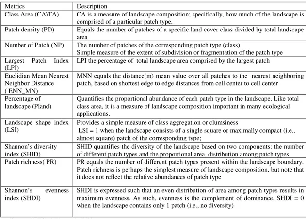
Spatial pattern analysis

Nearest Neighbor Distance(EMN_NN), Mean Patch Fractal Dimension (FRAC_AM), Patch Richness(PR), Shannon’s Diversity Index (SHDI), Shannon’s Evenness Index(SHEI) which have already been used in different studies (Herold et al., 2003) were adopted and used (Table 5). These metrics describe the composition and configuration of landscape pattern and also used to measure, the landscape fragmentation, dominancy, and diversity. The metrics were computed for each land cover map of 1987, 1995 and 2003 at the class and landscape level. Even though many of the class and landscape indices represent the same fundamental information, class indices represent the spatial distribution and pattern within a landscape of a single patch type; landscape indices represent the spatial pattern of the entire landscape mosaic, considering all patch types simultaneously. All these metrics were calculated using the FRAGSTAT software3.3 public domain software (McGarigal et al., 2002).

Table 5 Class and landscape metrics adopted and used in this study

Metrics Description

Class Area (CA\TA) CA is a measure of landscape composition; specifically, how much of the landscape is comprised of a particular patch type.

Patch density (PD) Equals the number of patches of a specific land cover class divided by total landscape area

Number of Patch (NP) The number of patches of the corresponding patch type (class)

Simple measure of the extent of subdivision or fragmentation of the patch type Largest Patch Index

(LPI)

LPI the percentage of total landscape area comprised by the largest patch

Euclidian Mean Nearest Neighbor Distance ( ENN_MN)

MNN equals the distance(m) mean value over all patches to the nearest neighboring patch, based on shortest edge to edge distances from cell center to cell center

Percentage of landscape (Pland)

Quantifies the proportional abundance of each patch type in the landscape. Like total class area, it is a measure of landscape composition important in many ecological applications.

Landscape shape index

(LSI) Provides a simple measure of class aggregation or clumsiness LSI = 1 when the landscape consists of a single square or maximally compact (i.e., almost square) patch of the corresponding type;

Shannon’s diversity index (SHID)

SHID quantifies the diversity of the landscape based on two components: the number of different patch types and the proportional area distribution among patch types Patch richness( PR) PR equals the number of different patch types present within the landscape boundary.

Patch richness is perhaps the simplest measure of landscape composition, but note that it does not reflect the relative abundances of patch type

Shannon’s evenness

index (SHDI) SHDI is expressed such that an even distribution of area among patch types results in maximum evenness. As such, evenness is the complement of dominance. SHDI = 0 when the landscape contains only 1 patch (i.e., no diversity)

5 RESULT AND DISCUSSION 5.1 Result

This chapter presents the result of LUCC change from classification of Landsat images and mainly focuses on result of classification accuracy assessment, analysis of the nature, extent and rate of land cover change, land use and cover change detection and spatial pattern of land cover dynamic.

5.1.1 Classification accuracy assessment

Table 6 Landsat TM classification accuracy for 1987

LC WL BL GR SGL BL CU SET UA%

WL 17 2 1 - - - - 85.00

BL 1 9 - - - 90.00

GR 3 - 25 2 - 2 - 83.33

SGR - - 1 6 1 - - 75.00

BL - - 3 10 - 1 71.43

CU - - - - 6 - 75.00

SET - - - - 1 - 5 83.33

RT 21 11 30 8 12 8 6

PA (%) 80.95 81.82 83.33 75.00 83.33 75.00 83.33 Kappa 0.80 0.89 0.75 0.73 0.66 0.73 0.82 Overall classification accuracy = 81.82%

Overall Kappa Statistics = 0.7671

WL: Woodland; BL: Bush land, GR: Grassland: SGR: Shrub grassland, BL: Bare land, CU: Cultivation: ST: Settlement, RF: Reference total, UA: User accuracy, PA: Producer accuracy

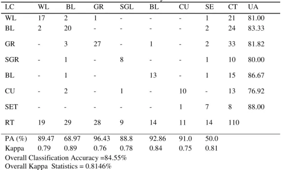
Table 7 Landsat TM classification accuracy for 1995

LC WL BL GR SGL BL CU SE CT UA

WL 17 2 1 - - - 1 21 81.00

BL 2 20 - - - - 2 24 83.33

GR - 3 27 - 1 - 2 33 81.82

SGR - 1 - 8 - - 1 10 80.00

BL - 1 - 13 - 1 15 86.67

CU - 2 - 1 - 10 - 13 76.92

SET - - - 1 7 8 88.00

RT 19 29 28 9 14 11 14 110

PA (%) 89.47 68.97 96.43 88.8 92.86 91.0 50.0 Kappa 0.79 0.89 0.76 0.78 0.84 0.75 0.81 Overall Classification Accuracy =84.55%

Overall Kappa Statistics = 0.8146%

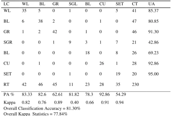
Table 8 Landsat TM classification accuracy for 2003

LC WL BL GR SGL BL CU SET CT UA

WL 35 5 0 1 0 0 5 41 85.37

BL 6 38 2 0 0 1 0 47 80.85

GR 1 2 42 0 1 0 0 46 91.30

SGR 0 0 1 9 3 1 7 21 42.86

BL 0 0 0 0 18 0 8 26 69.23

CU 0 1 0 0 0 26 1 28 92.86

SET 0 0 0 1 0 0 19 20 95.00

RT 42 46 45 11 23 28 35 230

PA % 83.33 82.6 62.61 81.82 78.3 92.86 54.29 Kappa 0.82 0.76 0.89 0.40 0.66 0.91 0.94 Overall Classification Accuracy = 81.30%

Overall Kappa Statistics = 77.84%

WL: Woodland; BL: Bush land, GR: Grassland: SGR: Shrub grassland, BL: Bare land, CU: Cultivation: SE: Settlement, RF: Reference total, UA: User accuracy, PA: Producer accuracy, CT: Classification total

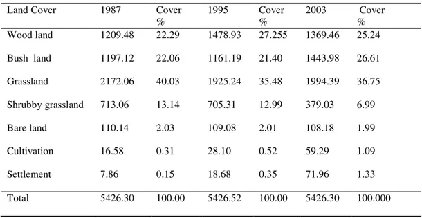
5.1.2 Land use and land cover classification 1987-2003

land, cultivation and settlement (Table 9). In 2003 Landsat ETM+ image showed that although grassland was the dominate land cover class, it had showed progressive reduction from 40.03 %( 1987) to 35.48 %( 2003) and followed by bush land 26.61% which showed rapid increment in the study area. Shrubby grassland cover about 6.98% of the area which indicated doubled fold reduction in cover from 13.14% to 6.99%. Although cultivation and settlement had covered small proportion of the study area, it had showed rapid increment. On the other hands, bare lands were showed little change (Table 9).

Table 9 Area statistics and percentage of the land use/cover units in 1987-2003

Land Cover 1987 Cover

% 1995 Cover % 2003 Cover % Wood land 1209.48 22.29 1478.93 27.255 1369.46 25.24

Bush land 1197.12 22.06 1161.19 21.40 1443.98 26.61

Grassland 2172.06 40.03 1925.24 35.48 1994.39 36.75

Shrubby grassland 713.06 13.14 705.31 12.99 379.03 6.99

Bare land 110.14 2.03 109.08 2.01 108.18 1.99

Cultivation 16.58 0.31 28.10 0.52 59.29 1.09

Settlement 7.86 0.15 18.68 0.35 71.96 1.33

Figure 9 Land use land cover classification map for 2003

In order to determine the magnitude, extent and rate of change of land use and land cover change dynamic in the study area, the following variables were calculated and used. These variables include Total Area (TA), Changed Area (CA), Change Extent (CE) and Annual Rate of change (CR). The variable was calculated as follows

CA=TA (t2)-TA (t1) CE= 100x [CA/TA (t1)] CR=CE/ (t2-t1)

Result indicated a rapid expansion of woodland cover was recorded between 1987 and 1995 (22.28%) (Table 10), but then declined between 1995 and 2003(5.24%). In overall, during 1987 to 2003, woodland had reduced by 11.68%. Similarly, the proportion of bush land had moderately reduced by 3%, in the earlier period (1987– 1995) than significantly increased to 24.84% in second period of studies (1995-2003). In general, over the years from 1987-2003 bush lands were increased by17.49% in the landscape. Grassland had showed rapid reduction (11.36%) in the first period than moderate increased during second period (4.81%). In overall, over the past 16-years rapid reduction of grassland (7.73%) cover in the savanna landscape was take place (Table 10). Unlike bush land, shrubby grassland showed significant reduction in the study period both in the first (1.09%) and second period of time (45.19%). In general, over 86.14% of reduction of shrubby grassland had been identified between 1987 and 2003. Bare land had showed little change over the past year from 1987 to 2003 and the change was consistence and less than 1%. Although cultivated area covered a small proportion of the landscape, rapid increment was observed over the past 16 years (72.49%) and dramatic increment had recorded in the second period of study (111.92%) than earlier time (69.52%). This suggesting that the Borana pastoralist have probably gradually shifted from a heavier dependence on livestock keeping to crop cultivation in some location.

Table 10 Overall amount, extent and rate of land cover change (1987-2003)

CA=Changed Area; CE=Changed Extent; CR=Annual rate of changed; WL: Woodland; BL: Bush land, GR: Grassland: SGR: Shrub grassland, BL: Bare land, CU: Cultivation: ST: Settlement

Figure 10 Nature of relative land cover changes 1987 to 2003

5.1.3 Change detection analysis

The LUCC change dynamic in Yabello, Ethiopia have detected and quantified by analyzing the classified multi-temporal satellite images of 1987, 1995 and 2003. A post classification comparison change detection algorithm was employed to

Land Cover

1987-1995 1995-2003 1987-2003

CA km2

CE %

CR %

CA km2

CE %

CR %

CA km2

CE %

CR %

determine change in land cover in time intervals, 1995, 1995-2003 and 1987-2003. This is the most common method to change detection. The post classification approach provides detailed “from-to”change information and the kind of landscape transitions that have occurred. In relation to this, change detection matrix of ‘from-to’ change was derived to show land cover class transition over the past 16-year. In relation to the transition matrix, net change, persistence and net change to persistence ratio (Braimoh, 2006; Pontius et al, 2004) were computed to show the resistance and vulnerability of a given land use and cover type using IDRIS ANDES Land Change Modeler. Furthermore, change detection using NDVI approaches was done to observe the trend of the vegetation greenness in the study area. The Table 11, 12 and 13 presented below is the change detection matrix that depicts what is changed to what. The column of the table represents the initial stage and the row represents the final stage. In this regard, image differencing was applied likewise from initial to final image. The diagonal values of the table shows the unchanged values, which are found in both times image. Unlike the diagonal values the class change tells the total changed image areas of each LUCC of the initial stages. Whereas the class total value of the column indicates the initial stage image total area of each LUCC classes where as the row total represents the final stage area of LUCC classes. The net change is the total net change of the two time images. The negative image change indicates a certain land use and land cover is in a state of decrement while the positive value indicates increment.

hand, woodland mainly converted from shrubby grassland (2.94%) (Figure 11). Bush land mainly increased at the expanse of grassland (1.79%) and shrubby grassland (0.79%). On the other hand, substantial amount of bush land was converted to cultivation (0.13) and settlement (0.23%) land type (Figure 11). Result also indicated that grassland (1.79%) had primarily converted to bush land and considerable amount of area was converted from woodland (0.51%). On the other hand, considerable proportion was gain from transformation of woodland (0.51%) (Figure11).Shrubby grassland mainly gained from grassland (0.17%). On the other hand extensive proportion of area was converted to woodland (2.94%) and bush land (0.79) (Figure 11 and Annex Table 4).

Table 11 Land-use/cover transition matrix showing major change in the landscape (km2), Yabelo, Ethiopia, 1987-2003

From initial state (1987)

To final state (2003)

WL BL GR SGL BL CU SET Total 2003

WL 389.23 311.72 342.15 304.79 19.93 1.32 0.29 1369.46

BL 354.26 366.81 524.89 167.09 28.42 1.88 0.61 1443.98

GR 388.61 361.29 1163.89 39.63 22.59 5.69 1.69 1994.39

SGR 35.71 94.71 55.41 178.35 13.35 1.30 0.19 379.03

BL 21.13 27.42 30.19 13.36 14.58 1.00 0.49 108.18

CU 4.59 13.75 27.15 7.26 5.75 4.46 0.32 59.29

SET 15.93 21.43 25.37 2.56 5.49 0.91 4.27 71.96

Total 1987 1209.49 1197.12 2172.07 713.06 110.14 16.58 7.86 2118.6(39%)

Gain 980.21 1077.17 827.51 200.68 93.59 58.82 71.7 Loss 820.24 830.31 1005.18 534.71 95.55 16.11 7.59 Net change 159.97 246.86 -177.67 -334.03 -1.95 42.71 64.1 Persistence 389.23 366.82 1166.88 178.35 14.59 0.46 2.27

Np 0.40 0.67 -0.15 -1.87 -0.13 9.6 15

WL: Woodland; BL: Bush land, GR: Grassland: SGR: Shrub grassland, BL: Bare land, CU: Cultivation: ST: Settlement. Np refers to net change to persistence ratio (i.e., net change/diagonals of each class, in ratio).The shaded figure is the sum of diagonals and represents the overall persistence (i.e., the landscape that did not change). Net change = gain−loss.

Wood land Bare land

Bush land Cultivation land

Grassland Settlement

Shrubby grassland

Table 12 Land-use/cover transition matrix showing major changes in the landscape (Km2_{), Yabelo,}

Ethiopia, 1987-1995

From initial

state (1987) _WL To final state (1995) _{BL GR SGL BL CU SET Total} 1995 WL 458.43 397.09 303.28 304.89 12.01 2.63 1.10 1478.93

BL 297.69 366.12 384.67 76.35 27.30 2.07 0.48 1161.19

GR 326.49 295.50 1175.47 71.16 44.46 4.43 1.73 1925.24

SGR 104.34 116.51 218.19 254.06 11.67 0.47 0.08 705.31

BL 11.78 13.64 67.34 2.21 10.10 2.10 1.91 109.08

CU 5.32 3.43 14.40 1.09 2.77 4.60 0.40 18.68

SET 4.20 3.46 6.40 2.66 1.65 0.23 3.08 28.10

Total 1987 1209.48 1197.12 2172.06 713.06 110.14 16.58 7.86 2272.04 (41.87)

Gain 1020.50 789.07 749.77 451.25 98.98 27.41 18.60

Loss 749.81 829.63 994.28 458.36 99.87 15.93 7.70

Net change 270.69 -40.56 - 244.51 -7.10 -0.90 11.48 10.91

Persistence 458.43 366.12 1175.47 254.06 10.10 4.60 2.08

NP 0.59 -0.11 -0.21 -0.03 -0.09 2.49 3.54

WL: Woodland; BL: Bush land, GR: Grassland: SGR: Shrub grassland, BL: Bare land, CU: Cultivation: ST: Settlement. Np refers to net change to persistence ratio

Wood land Bare land

Bush land Cultivation land

Grassland Settlement

Shrubby grassland

Land use change detection and net contribution by each land use class for 1995-2003 is presented in Table 13 and Figure 13. Based on the analysis, woodland, shrubby grassland and bare land had continuously decreased by 110.82, 326.65 and 0.94 km2, respectively. On the other hand, grassland, bush land, settlement and cultivations were increased by 287.30, 66.62, 31.25 and 53.24 km2 areas, respectively. The highest net change was observed in shrubby grassland while the lowest was identified in bare land (0.94) (Table 13). Between 1995 to 2003 woodland in the landscape converted to all land use type (Figure 12).This indicating that there was human activities on woodland. Result also indicated that bush land was mainly converted to woodland. From Figure 13 grassland mainly increase at expense of shrub grassland. Similar, cultivation mainly increases at the expanse of shrubby grassland while settlement was mainly converted from grassland (Figure 12 and Annex Table 4). The net change-to persistence ratio of bush land, grassland, cultivation and settlement was showed positive trend. On the other hand, woodland, shrubby grassland, and bare land had negative trend in the changing landscape. Overall, 42.42% of the total landscape remains unchanged (Table 13).

Table 13 Land-use/cover transition matrix showing major changes in the landscape (km2), Yabelo, Ethiopia, 1995-2003

From initial state (1995)

To final state (2003)

WL BL GR SGL BL CU SET To final state (2003)

WL 679.79 236.14 164.10 283.019 3.10 1.039 0.92 1369.46

BL 374.67 396.98 461.63 191.478 8.85 4.149 4.73 1443.98

GR 258.91 405.69 1108.82 120.45 69.82 7.91 3.28 1994.39

SGR 139.83 66.838 69.59 91.83 5.53 2.35 2.10 379.03

BL 17.86 18.167 46.00 6.86 13.37 3.35 2.03 108.18

CU 6.28 18.503 35.62 1.72 6.00 6.84 1.12 59.29

SET 1.59 12.875 30.48 9.96 2.40 0.04 5.42 71.96

Total 1478.93 1161.19 1925.24 705.31 109.08 28.10 18.68 2303(42.42)

Gain 688.32 1045.50 874.04 286.83 94.76 70.51 58.43 Loss 799.14 758.20 807.42 613.48 95.71 17.26 27.18 Net change -110.82 287.30 66.62 -326.65 -0.94 53.24 31.25 Persistence 679.79 396.98 1108.82 91.83 13.37 6.84 5.42

NP -0.16 0.72 0.06 -0.26 -0.07 7.78 3.45

Wood land Bare land

Bush land Cultivation land

Grassland Settlement

Shruby grassland