BAYES AHMED
URBAN LAND COVER CHANGE DETECTION
ANALYSIS AND MODELLING SPATIO-TEMPORAL
GROWTH DYNAMICS USING REMOTE SENSING
AND GIS TECHNIQUES
URBAN LAND COVER CHANGE DETECTION ANALYSIS AND
MODELLING SPATIO-TEMPORAL GROWTH DYNAMICS
USING REMOTE SENSING AND GIS TECHNIQUES
“A CASE STUDY OF DHAKA, BANGLADESH”
Dissertation Supervised by
Dr. Pedro Latorre Carmona
Professor, Institute of New Imaging Technologies (INIT)
Universitat Jaume I (UJI), Castellón, Spain
Dissertation Co-Supervised by
Dr. Mário Caetano
Professor, Instituto Superior de Estatística e Gestão de Informação (ISEGI)
Universidade Nova de Lisboa (UNL), Lisbon, Portugal
Dr. Edzer Pebesma
Professor, Institute for Geoinformatics (ifgi)
Westfälische Wilhelms-Universität (WWU), Münster, Germany
Dr. Nilanchal Patel
Professor, Department of Remote Sensing
Birla Institute of Technology Mesra, Jharkhand, India
Candidate’s Declaration
This is to certify that this research work is entirely my own and not of any other person, unless explicitly acknowledged (including citation of published and unpublished sources).
All views and opinions expressed therein remain the sole responsibility of the author, and do not necessarily represent those of the institutes.
It is hereby also declared that this dissertation or any part of it has not been submitted elsewhere for the award of any degree or diploma.
_____________________________
BAYES AHMED
Dedication
I want to dedicate this research work to
My beloved Parents
Md. Abdus Sattar
and
i
Abstract
Dhaka, the capital of Bangladesh, has undergone radical changes in its physical form, not only in its vast territorial expansion, but also through internal physical transformations over the last decades. In the process of urbanization, the physical characteristic of Dhaka is gradually changing as open spaces have been transformed into building areas, low land and water bodies into reclaimed builtup lands etc. This new urban fabric should be analyzed to understand the changes that have led to its creation.
The primary objective of this research is to predict and analyze the future urban growth of Dhaka City. Another objective is to quantify and investigate the characteristics of urban land cover changes (1989-2009) using the Landsat satellite images of 1989, 1999 and 2009. Dhaka City Corporation (DCC) and its surrounding impact areas have been selected as the study area. A fisher supervised classification method has been applied to prepare the base maps with five land cover classes. To observe the change detection, different spatial metrics have been used for quantitative analysis. Moreover, some post-classification change detection techniques have also been implemented. Then it is found
that the ‘builtup area’ land cover type is increasing in high rate over the years. The major
contributors to this change are ‘fallow land’ and ‘water body’ land cover types.
In the next stage, three different models have been implemented to simulate the land
cover map of Dhaka city of 2009. These are named as ‘Stochastic Markov (St_Markov)’ Model, ‘Cellular Automata Markov (CA_Markov)’ Model and ‘Multi Layer Perceptron Markov (MLP_Markov)’ Model. Then the best-fitted model has been selected based on various Kappa statistics values and also by implementing other model validation
techniques. This is how the ‘Multi Layer Perceptron Markov (MLP_Markov)’ Model has
been qualified as the most suitable model for this research. Later, using the MLP_Markov model, the land cover map of 2019 has been predicted. The MLP_Markov model shows that 58% of the total study area will be converted into builtup area cover type in 2019.
The interpretation of depicting the future scenario in quantitative accounts, as demonstrated in this research, will be of great value to the urban planners and decision makers, for the future planning of modern Dhaka City.
ii
Acknowledgement
At the outset, all praises belong to the almighty ‘Allah’, the most merciful, the most beneficent to all the creatures and their dealings.
First of all, I would like to express my gratitude to the European Commission and Erasmus Mundus Consortium (Universitat Jaume I, Castellón, Spain; Westfälische Wilhelms-Universität, Münster, Germany and Universidade Nova de Lisboa, Portugal) for awarding me the Erasmus Mundus scholarship in Master of Science in Geospatial Technologies. It is a great opportunity for my lifetime experiences to study in the reputed universities of Europe.
It is a great pleasure to acknowledge my sincere and greatest gratitude to my dissertation supervisor, Dr. Pedro Latorre Carmona, Professor, Institute of New Imaging Technologies, University Jaume I, Spain; for his untiring effort, careful supervision, thoughtful suggestions and enduring guidance at every stage of this research. This thesis would not be in its current shape without his continuous exertion and support.
I am very grateful to my dissertation co-supervisors Dr. Mário Caetano, Dr. Edzer Pebesma and Dr. Nilanchal Patel; for accepting my thesis proposal at the very early stage and also for their valuable time and effort in contributing information and practical suggestions on numerous occasions.
My heartfelt thanks goes to Dr. Raquib Ahmed, Professor and Director, Institute of Environmental Science, University of Rajshahi, Bangladesh; for his initial encouragement for conducting this research and helping me developing the research proposal.
I also want to thank Dr. Filiberto Pla Bañón, Professor, Institute of New Imaging Technologies, Universitat Jaume I, Spain; for his time and some comments. I am pleased to extend my gratitude to Prof. Dr. Joaquín Huerta Guijarro, Dolores C. Apanewicz, Prof. Dr. Jorge Mateu and Dr. Christoph Brox; for their support and hospitality during my stay in Spain and Germany.
My thanks and best wishes also conveyed to my classmates and lovely friends, from all over the world, for sharing their knowledge and giving me inspirations during the last eighteen months in Europe. Special thanks goes to Dipu da, Anik vai, Shiuli vabi, Irene, Mauri, Carlos, Sherzod, Neba, Shahin vai, Diyan vai, Pathak, Freska and Pearl for their patronage and helping me coping with this new and challenging European environment.
iii
Index of the Text
Content
Page No
Abstract i
Acknowledgement ii
Index of the Text iii
Index of Figures viii
Index of Tables x
Abbreviations and Acronyms xii
Chapter 1: Introduction
1.1 Background of the Research 1
1.2 Statement of the Problem 1
1.3 Study Area Profile 5
1.4 Objectives of the Research 9
1.5 Research Hypotheses 9
1.5.1 Related to Objective 1 9
1.5.2 Related to Objective 2 9
1.6 Limitations of the Research 10
1.6.1 Collection of Satellite Images 10
1.6.2 Seasonal Variation 10
1.6.3 Collection of Reference Data 10
Chapter 2: Theoretical Framework and Methodology
2.1 Basic Terminologies 11
2.1.1 Remote Sensing (RS) 11
2.1.2 Geographic Information System (GIS) 11
2.1.3 Land 12
2.2 Literature Review 12
2.2.1 Examples Related to Land Cover Change Detection 13 2.2.2 Examples Related to Future Land Cover Prediction 14
iv
2.3.1 Selection of Study Area 14
2.3.2 Problem Identification and Research Objectives 14
2.3.3 Data Collection 16
2.3.3.1 Satellite Images 16
2.3.3.2 Reference Data 18
2.3.3.3 Literature Review 18
2.3.4 Base Map Preparation and Accuracy Assessment 18
2.3.5 Change Detection Analysis 18
2.3.6 Model Calibration/ Simulation 18
2.3.7 Model Validation and Selection 19
2.3.8 Future Prediction 19
2.3.9 Directions for Future Planning 19
2.3.10 Report Writing 19
2.4 Tools Used for this Research 19
Chapter 3: Base Map Preparation and Accuracy Assessment
3.1 Image Enhancement 20
3.2 Composite Generation 20
3.3 Image Classification 22
3.3.1 Training Site Development 22
3.3.2 Signature Development 24
3.3.3 Classification 24
3.3.4 Generalization 24
3.4 Accuracy Assessment 26
3.4.1 Assessment Procedure 27
3.4.2 Results and Discussion 30
Chapter 4: Land Cover Change Detection Analysis
4.1 Change Detection 31
4.2 Terminologies 31
v
4.3.4 Change in Area 35
4.3.5 Gains and Losses by Category 35
4.3.6 Contributors to Net Change Experienced by Builtup Area 36
4.3.7 Transition to Builtup Area 36
4.3.8 Gains and Losses in Land Cover Types 38
4.4 Summary of Land Cover Change Detection Analysis 38
Chapter 5: Stochastic Markov Model
5.1 Stochastic Process 40
5.2 Markov Chain 40
5.2.1 Markov Property 41
5.2.2 Transition Matrix for a Markov Chain 41
5.2.3 Example of Markov Chain 42
5.2.3.1 Weather Prediction 43
5.3 Stochastic Markov Model 43
Chapter 6: Cellular Automata Markov Model
6.1 Cellular Automata 48
6.1.1 What are Cellular Automata? 48
6.1.2 The Elements of Cellular Automata 48
6.1.3 The Cell Space 49
6.1.4 The Cell States 50
6.1.5 The Cell Neighbourhood 50
6.1.6 The Transition Rules 51
6.1.7 The Temporal Space 52
6.1.8 Mathematical Notation of Cellular Automata 52
6.1.9 Running a Simulation 53
6.2 Cellular Automata Markov Model 54
6.3 How CA_Markov Model Works? 54
6.3.1 Suitability Maps for Land Cover Classes 56
6.3.2 Preparing Suitability Maps 57
vi
Chapter 7: Multi Layer Perceptron Markov Model
7.1 Artificial Neural Network 64
7.2 Basic Concept of Artificial Neural Network (ANN) 64
7.2.1 Types of Artificial Neural Network 65
7.3 Multi Layer Perceptron (MLP) 65
7.3.1 Input Layer 66
7.3.2 Hidden Layer 66
7.3.3 Output Layer 66
7.3.4 The Feed-Forward Concept of MLP Neural Network 67
7.3.5 Number of Nodes 68
7.3.6 Number of Training Samples and Iterations 68
7.4 Multi Layer Perceptron Markov Modelling 69
7.4.1 Testing Potential Explanatory Power 72
7.4.2 Transition Potential Modelling 73
7.4.3 Future Prediction 75
Chapter 8: Model Validation and Selection
8.1 Model Validation 76
8.1.1 Per Category Method 77
8.1.2 Fraction Correct 78
8.1.3 Fuzzy Sets 78
8.1.4 Fuzzy Kappa 79
8.2 Actual Base Maps vs. Simulated Maps 81
8.2.1 Base Map (2009) vs. St_Markov (2009) 81
8.2.1.1 Analysis of the Results of St_Markov 84
8.2.2 Base Map (2009) vs. CA_Markov (2009) 85
8.2.2.1 Analysis of the Results of CA_Markov 88
8.2.3 Base Map (2009) vs. MLP_Markov (2009) 89
8.3 Model Selection 91
Chapter 9: Future Prediction and Analysis
9.1 Future Prediction 92
9.1.1 Creating Boolean Images (2009) 92
vii
9.1.3 Creating Land Cover Transition Image 94
9.1.4 Selecting Driving Variables 94
9.1.5 Testing Potential Explanatory Power of the Driving Variables 96
9.1.6 Transition Potential Modelling 96
9.1.7 Markov Chain Analysis 98
9.2 Analysis of the Predicted Map 99
9.3 Limitations of MLP_Markov Model 99
Chapter 10: Recommendations and Conclusions
10.1 Answers to Research Questions 101
10.1.1 Answers Related to Objective 1 101
10.1.2 Answers Related to Objective 2 101
10.2 Recommendations for Future Work 102
10.3 Recommendations for Real World Plan Preparation 103
10.4 Epilogue 104
References
105Appendices
Appendix A: Photographs: Some Existing Urban Problems within Dhaka City 113
Appendix B: Reference Maps 114
Appendix C: Details of Accuracy Assessment 117
C 1 Basic Terminologies 117
C 1.1 Ground Truth 117
C 1.2 Overall Accuracy 117
C 1.3 Producer’s Accuracy 117
C 1.4 User’s Accuracy 117
C 1.5 Kappa 118
C 1.6 Kno 120
C 1.7 Klocation 121
C 1.8 Khisto 121
C 2 Accuracy Assessment Report 122
viii
Appendix D: Terminologies Used for Land Cover Change Detection Analysis 125
D 1 Patch 125
D 2 Landscape 125
D 3 Core Area 125
D 4 Number of Patches (NP) 126
D 5 Edge Density (ED) 126
D 6 Largest Patch Index (LPI) 126
D 7 Core Area Percentage of Landscape (CPLAND) 127 D 8 Mean Euclidean Nearest-Neighbour Distance (ENN_MN) 127
D 9 Mean Fractal Dimension Index (FRAC_MN) 127
Appendix E: Quantitative Values for Change Detection Analysis 128 Appendix F: Summary of Land Cover Classification Statistics (1989 - 2009) 129
Appendix G: Land Use Suitability 130
G 1 Land Use Suitability Analysis 130
G 2 Different Methods for Land Use/Cover Suitability Analysis 130 G 2.1 Computer-Assisted Overlay Mapping Technique 130 G 2.2 Multi Criteria Decision Making Methods 130 G 2.3 Artificial Intelligence (AI) Methods 131
Appendix H: Sigmoid Function and Cramer’s V 132
H 1 Sigmoid Function 132
H 2 Cramer’s V 132
Index of Figures
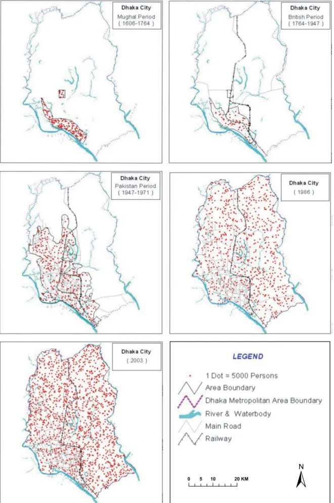
Figure 1.1: Changing Patterns of Dhaka City in Area and Population 3 Figure 1.2: Satellite Images Showing Urban Growth of Dhaka 6
Figure 1.3: Location of Dhaka City 7
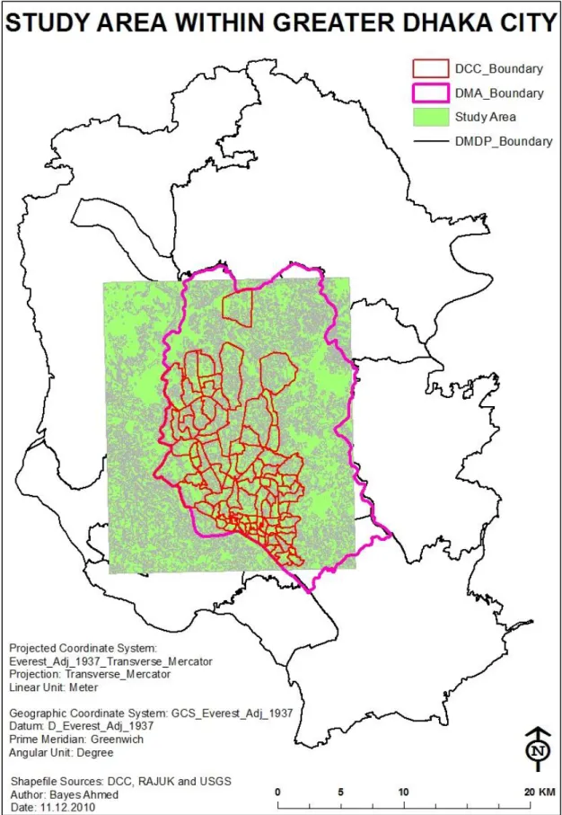
Figure 1.4: Location of the Study Area within Greater Dhaka City 8
Figure 2.1: Flow Chart of Methodology 15
Figure 2.2: Dhaka City Corporation and its Surroundings 17 Figure 3.1: Composites Using Different Band Combinations 20 Figure 3.2: False Color Composite (RGB=4, 3 and 2) Maps 21
Figure 3.3: Land Cover Maps of Dhaka City 25
ix
Figure 3.5: Selected Stratified Random Points for Ground Truthing 29 Figure 4.1: Number of Patches and Largest Patch Index 32 Figure 4.2: Edge Density and Mean Fractal Dimension Index 33
Figure 4.3: ENN_MN and CPLAND 34
Figure 4.4: Land Cover Change in Area (Percentage) 35 Figure 4.5: Gains and Losses of Land Covers by Category 36 Figure 4.6: Contributors to Net Change Experienced by Builtup Area 37 Figure 4.7: Transition of Other Land Cover Types into Builtup Area 37 Figure 4.8: Gains and Losses in Land Cover Types (1989-2009) 39
Figure 5.1: Example of a Markov Chain 41
Figure 5.2: Stochastic Weather Model 43
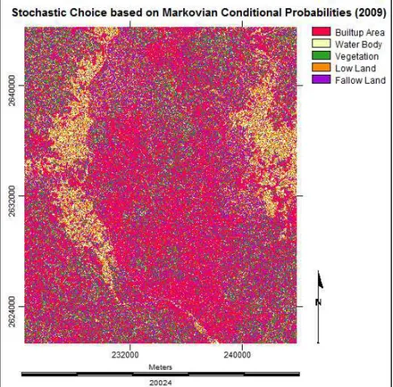
Figure 5.3: Markovian Conditional Probability Images 45 Figure 5.4: Stochastic Markov Predicted Land Cover Map (2009) 47 Figure 5.5: Final St_Markov Predicted Land Cover Map (2009) 47
Figure 6.1: One-Dimensional Cellular Automata 49
Figure 6.2: Two-Dimensional Cellular Automata Grid 49
Figure 6.3: Examples of Variegated Cells 50
Figure 6.4: Two-Dimensional CA Neighbourhoods 51
Figure 6.5: The 3 × 3 Mean Contiguity Filter for CA_Markov Modelling 55
Figure 6.6: Fuzzy Linear Membership Function 58
Figure 6.7: Boolean Images of each Land Cover Type (1999) 59 Figure 6.8: Distance Images of each Land Cover Type (1999) 60 Figure 6.9: Suitability Images of each Land Cover Type 61 Figure 6.10: Aggregated Land Cover Suitability Map of Dhaka City (1999) 62 Figure 6.11: CA_Markov Projected Land Cover Map of Dhaka City (2009) 63 Figure 7.1: Artificial Neural Network Processing Element 64 Figure 7.2: A Multi Layer Perceptron Neural Network Model 65 Figure 7.3: Working Methodology of a Neuron in MLP Network 66 Figure 7.4: Transitions of Land Covers between 1989 and 1999 69 Figure 7.5: Transition from All to Builtup Area (1989-1999) 70 Figure 7.6: Distance Image of Transition from All to Builtup Area 71 Figure 7.7: Empirical Likelihood Image (1989-1999) 71
Figure 7.8: RMS Error Monitoring Curve 73
x
Figure 7.10: MLP_Markov Projected Land Cover Map of Dhaka City 75
Figure 8.1: Cell-by-cell Map Comparison 76
Figure 8.2: Cell-by-cell Map Comparison of Two Maps 77 Figure 8.3: Per Category Map Comparison of Two Maps 78 Figure 8.4: Fuzzy vs. Crisp Set Membership Functions 79
Figure 8.5: Difference between ‘Cell-by-cell’ and ‘Fuzzy’ Comparison 80 Figure 8.6: Levels of Agreement for Fuzzy Comparison Method 80
Figure 8.7: Maps for Model Validation 81
Figure 8.8: Levels of Agreement for Kappa 82
Figure 8.9: Per Category Comparison Method 83
Figure 8.10: Maps for Model Validation 85
Figure 8.11: Levels of Agreement for Kappa 85
Figure 8.12: Per Category Comparison Method 86
Figure 8.13: Fuzzy Kappa Result Map 87
Figure 8.14: Maps for Model Validation 89
Figure 8.15: Levels of Agreement for Kappa 89
Figure 8.16: Per Category Comparison Method 90
Figure 9.1: Boolean Images of each Land Cover Type (2009) 92 Figure 9.2: Distance Images of each Land Cover Type (2009) 93 Figure 9.3: Transition from All to Builtup Area (1999-2009) 94 Figure 9.4: Distance Image of Transition from All to Builtup Area 95 Figure 9.5: Empirical Likelihood Image (1999-2009) 95
Figure 9.6: RMS Error Monitoring Curve 97
Figure 9.7: Transition Potential Maps 97
Figure 9.8: MLP_Markov Projected Land Cover Map of Dhaka City 98 Figure 9.9: Change in Area (%) over the Years (1989-2019) 99 Figure 9.10: Gains and Losses of Land Cover Types (2009-2019) 100
Figure D 1: Classes of Landscape Pattern 125
Figure H 1: Sigmoid Function 132
Index of Tables
Table 1.1: Growth of Dhaka City in Urban Agglomerations (1950-2025) 2 Table 1.2: Historical Growth of Dhaka City in Terms of Area 4
xi
Table 3.1: Properties of the Processed Raster Images for Analysis 23
Table 3.2: Details of the Land Cover Types 23
Table 3.3: Accuracy Assessment Cell Array 28
Table 5.1: Markov Probability of Changing among Land Cover Types 44 Table 5.2: Cells Expected to Transition to Different Classes 44 Table 5.3: Stochastic Random Process for Selecting Land Cover Type 46 Table 6.1: The Factor Weights Evaluated for the Suitability Map (1999) 62
Table 7.1: Cramer’s V of the Driving Factors 72
Table 7.2: Running Statistics of MLP Neural Network 73 Table 7.3: Transition Probabilities Grid for Markov Chain 75
Table 8.1: Per Category Land Cover Change 82
Table 8.2: Per Category Kappa Statistics 84
Table 8.3: Fuzzy Kappa per Category 87
Table 8.4: Per Category Land Cover Change 88
Table 8.5: Per Category Kappa Statistics 88
Table 8.6: Per Category Kappa Statistics 91
Table 8.7: Overall Kappa Statistics and Fraction Correct 91
Table 9.1: Cramer’s V of the Driving Factors 96
Table 9.2: Running Statistics of MLP Neural Network 96 Table 9.3: Transition Probabilities Grid for Markov Chain 98
Table C 1: An Example of Error Matrix 118
Table C 2: Contingency Table 119
Table C 3: Strength of Agreement for Kappa Statistic 120
Table C 4: Error Matrix (1989) 122
Table C 5: Accuracy Totals (1989) 122
Table C 6: Conditional Kappa for each Category (1989) 122
Table C 7: Error Matrix (1999) 123
Table C 8: Accuracy Totals (1999) 123
Table C 9: Conditional Kappa for each Category (1999) 123
Table C 10: Error Matrix (2009) 124
Table C 11: Accuracy Totals (2009) 124
xii
Abbreviations and Acronyms
AHP Analytical Hierarchy Analysis
AI Artificial Intelligence
ANN Artificial Neural Network
BBS Bangladesh Bureau of Statistics
BTM Bangladesh Transverse Mercator
BUET Bangladesh University of Engineering and Technology
CA Cellular Automata
CA_Markov Cellular Automata Markov Model
CPLAND Core Area Percentage of Landscape
DAP Detail Area Plan
DCC Dhaka City Corporation
DMA Dhaka Metropolitan Area
DMDP Dhaka Metropolitan Development Plan
DSMA Dhaka Statistical Metropolitan Area
ED Edge Density
EIU Economist Intelligence Unit
ENN_MN Mean Euclidean Nearest Neighbour Distance
ETM+ Enhanced Thematic Mapper Plus
FAO Food and Agriculture Organization
FRAC_MN Mean Fractal Dimension Index
xiii
GoB Government of the People’s Republic of Bangladesh
GPS Global Positioning System
LPI Largest Patch Index
MCDM Multi Criteria Decision Making
MCE Multi Criteria Evaluation
MLP Multi Layer Perceptron
MLP_Markov Multi Layer Perceptron Markov Model
MOLA Multi Objective Land Allocation
NASA National Aeronautics and Space Administration
NDVI Normalized Differential Vegetation Index
NP Number of Patches
OWA Ordered Weighted Averaging
RAJUK Rajdhani Unnayan Kartripakkh [Bangla] (Capital City Planning
and Development Authority)
RS Remote Sensing
SoB Survey of Bangladesh
St_Markov Stochastic Markov Model
TM Thematic Mapper
UAP Urban Area Plan
USGS United States Geological Survey
UTM Universal Transverse Mercator
WGS World Geodetic System
Chapter 1 1
Chapter 1
Introduction
1.1 Background of the Research
Urbanization is one of the most evident human induced global changes worldwide. In the past 200 years, the world population has increased 6 times and the urban population has multiplied 100 times [1].
Like many other cities in the world Dhaka, the capital of Bangladesh, is also the outcome of spontaneous rapid growth without any prior or systematic planning. As the growth of population in Dhaka is taking place at an exceptionally rapid rate, it has become one of the most populous Mega Cities1 in the world.
Dhaka City has undergone radical changes in its physical form, not only in its vast territorial expansion, but also through internal physical transformations over the last decades. These have created entirely new kinds of urban fabric.
In the process of urbanization, the physical characteristics of Dhaka City are gradually changing as plots and open spaces have been transformed into building areas, open squares into car parks, low land and water bodies into reclaimed built-up lands etc.
This new urban fabric is to be analyzed to understand the changes that have led to its creation. Therefore it is necessary to track the changes of modern Dhaka City which mainly includes the changes in the physical form of the city.
1.2 Statement of the Problem
Dhaka is enriched with rich culture, history and heritage of about 400 years [2, 3]. Dhaka was worldwide famous for its fine Muslin (a kind of very smooth cloth), mosques and trade [4, 5]. But the scenario has been changed over the centuries.
1 The term „Mega City‟ is frequently used as a synonym for words such as supe
Chapter 1 2 Dhaka is now attracting a huge amount of rural-urban migrants from all over the country due to well-paid job opportunities, better educational, health and other daily life facilities [7]. This kind of increasing and over population pressure is putting adverse impacts on Dhaka city like converting wetlands/natural vegetation/open space/bare soil to urban built-up areas [8, 9]. All these are creating numerous problems like unplanned urbanization, extensive urban poverty, water logging, growth of urban slums and squatters, traffic jam, environmental pollution and other socio-economic problems [7].
Dhaka has turned into one of the world’s biggest megacities [1]. Dhaka is now one of the world’s most populous, most densely populated and most urban agglomerated2 cities [10, 11, and 12]. According to the World Bank Annual Report (2007), Dhaka is going to
be world’s third largest city by 2020. The overall scenario of physical growth of Dhaka City has been depicted in Table 1.1, Figure 1.1 and Table 1.2.
Table 1.1: Growth of Dhaka City in Urban Agglomerations with 750,000
Inhabitants or More (1950-2025)
Source: Population Division of the Department of Economic and Social Affairs of the United Nations Secretariat, World Population Prospects: The 2008 Revision and World Urbanization Prospects: The 2009 Revision, http://esa.un.org/wup2009/unup/, retrieved on Wednesday, January 05, 2011.
Year
City Population (Thousands)
Urban Population Residing in Each Agglomeration (%)
Total Population Residing in Each Agglomeration (%)
Average Annual Rate of Change
(%)
1950 336 18.0 0.8
3.94 (1950-1955)
1955 409 18.0 0.8
1960 508 18.3 0.9 4.34 (1955-1960)
1965 821 21.7 1.3 9.60 (1960-1965)
1970 1374 26.2 2.0 10.30 (1965-1970)
1975 2221 28.6 2.8 9.61 (1970-1975)
1980 3266 24.3 3.6 7.71 (1975-1980)
1985 4660 25.9 4.5 7.11 (1980-1985)
1990 6621 28.9 5.7 7.02 (1985-1990)
1995 8332 30.0 6.5 4.60 (1990-1995)
2000 10285 31.0 7.3 4.21 (1995-2000)
2005 12555 31.9 8.2 3.99 (2000-2005)
2009 14251 31.9 8.8 3.08 (2005-2010)
2010 14648 31.7 8.9 2.53 (2010-2015)
2015 16623 30.8 9.5 2.38 (2015-2020)
2020 18721 29.8 10.1
2.24 (2020-2025)
Chapter 1 3
±
Figure 1.1: Changing Patterns of Dhaka City in Area and Population
Chapter 1 4
2 The term “Urban Agglomeration” refers to the population contained within the contours of a
contiguous territory in-habited at urban density levels without regard to administrative boundaries. It usually incorporates the population in a city or town plus that in the suburban areas lying outside of but being adjacent to the city boundaries [13].
Table 1.2: Historical Growth of Dhaka City in Terms of Area
Year Area (sq.km)
1600 1
1608 2
1700 40
1800 4.5
1867 10
1872 20
1881 20
1891 20
1901 20
1931 20
1941 25
1951 85
1961 125
1974 336
1981 510
1991 1353
2001 1530
Source: Taylor, J., Sketch of the Topography and Statistics of Dacca (Calcutta: Military Orphan Press, 1840); Bangladesh Bureau of Statistics (BBS), Bangladesh National Population Census Report - 1974 (Dhaka: Ministry of Planning, 1977); Bangladesh Population Census 1991 Urban Area Report (Dhaka: Ministry of Planning, 1997); Population Census 2001 Preliminary Report (Dhaka: Ministry of Planning, 2001) and [10, 14, 15].
If the trend of urbanization (in terms of population and area) of Dhaka is analyzed over time, then it is clear how spontaneously the city is growing (Table 1.1, 1.2 and Figure 1.1). The increase in population and area is degrading the living standard of Dhaka city.
Chapter 1 5 All these are really a matter of special consideration. If this situation continues then Dhaka would soon become an urban slum with the least liveable situation for the city dwellers. Moreover, the land cover3 pattern of Dhaka city is changing from vegetation (green) to builtup areas (brown) gradually (Figure 1.2). In this regard, it is much needed to track the land cover changes over-time and predict the future scenario of Dhaka city. This kind of research would be of great importance for the politicians, decision-makers and urban planners of Bangladesh to take early steps towards facing the worst situations about Dhaka city.
Some photographs depicting the existing urban life problems, due to this haphazard urban growth, of Dhaka city are presented in Appendix A.
1.3 Study Area Profile
There are 64 districts in Bangladesh. Dhaka City is located in Dhaka District that is surrounded by rivers. Dhaka is located in central Bangladesh at 23°43′0″N, 90°24′0″E, on the eastern banks of the Buriganga River [17]. Dhaka city area is under jurisdiction of different authorities that are known as Dhaka City Corporation (DCC), Dhaka Metropolitan Area (DMA), Dhaka Statistical Metropolitan Area (DSMA) and Dhaka Metropolitan Development Plan (DMDP) area. DCC comprises of 90 wards4 (Figure 1.3).
The proposed study area for this research is Dhaka City Corporation (DCC) and its surrounding impact areas (Figure 1.4). The study area covers the oldest organic core part of Dhaka city (old Dhaka), the planned areas and even the unplanned new generation organic areas that are called ‘Informal Settlements’. This selected study area almost covers the biggest urban agglomeration and is the central part of Bangladesh in terms of social and economic aspects [8, 10]. Therefore, this area has huge potentiality to face massive urban growth in near future based on the current trend of rapid urbanization.
3„
Land Cover‟ describes the physical state of the earth‟s surface and immediate subsurface in terms of the natural environment (such as vegetations, soils, surfaces and groundwater) and the man-made structures (e.g. buildings). While „Land Use‟ relates to the manner in which the biophysical assets are used by humans. „Land Use‟ is the human employment of a land-cover type [18, 19].
4„
Chapter 1 6
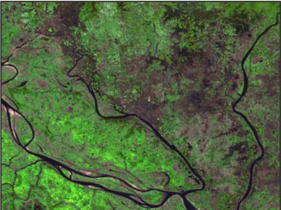
Figure 1.2: Satellite Images Showing Urban Growth of Dhaka (1972 to 2001) a. Dhaka on 28-12-1972 taken by Landsat-1-MSS
b. Dhaka on 13-02-1989 taken by Landsat-5-TM showing further growth since 1972
c. Dhaka on 29-01-2001 taken by Landsat-7-ETM+ showing further urban growth since 1989
Chapter 1 7
Figure 1.3: Location of Dhaka City
Chapter 1 8
Chapter 1 9
1.4 Objectives of the Research
The general objective of this research is to map, detect, quantify, analyze and predict the land cover changes of Dhaka City over time. For this reason, various existing modelling techniques have been implemented with the help of some spectral and multi-temporal remotely sensed and other geospatial datasets. The primary objective is to forecast the future urban land cover change of the selected study area within Dhaka city.
To address the above mentioned problems (section 1.2), this research has been conducted to achieve the following two broad objectives:
1. To quantify and investigate the characteristics of urban land cover changes (1989-2009) within the study area using satellite images.
2. To predict and analyze the future urban growth of Dhaka City.
1.5 Research Hypotheses
The following research questions or hypotheses have been considered to fulfil the above mentioned research objectives:
1.5.1 Related to Objective 1
1. Which datasets are available to conduct the whole research?
2. Which techniques are available for analyzing the change detection of land cover types of Dhaka city?
3. What is the general trend of land cover changes of the study area over time (1989-2009)?
1.5.2 Related to Objective 2
1. Which methods are available to simulate the future urban growth of the study area?
2. Which method is suitable for forecasting the future land cover changes?
3. Are the satellite images, GIS and Remote Sensing tools and different methods/ techniques used for this research adequate or useful?
Chapter 1 10
1.6 Limitations of the Research
1.6.1 Collection of Satellite Images
To perform this type of Spatio-temporal analysis, it is important to select the satellite images of the same time interval. Again the spatial resolution of the images is important. For this research purpose, Landsat satellite images have been chosen that are only commercially available but can be found in free public-domain. Another reason for choosing these images is that the time interval is found equal 10 years of interval (1989, 1999, and 2009). The main problem of working with Landsat images is low resolution. The spatial resolution of Landsat Image is 30 meter [21]. IKONOS, QuickBird or other satellite images with higher resolution can be better option, but those images are commercial. Therefore due to limitations of resources, only free public-domain data have been used for this research.
1.6.2 Seasonal Variation
Another important point, while selecting satellite images, is seasonal variation. Seasonal variation is an important aspect for tropical countries like Bangladesh. The change in vegetation, wet land, low land and water body land cove types are evident due to different seasons. Therefore, in an ideal situation, satellite images of the same season are selected for this kind of research. But there exist some sorts of seasonal variation for Landsat satellite images collected for this research. The images collected for 1999 (November) and 2009 (October) are from the same winter season. But the image of 1989 (February) is from another season, summer. This kind of variation creates problems while preparing base maps for analysis.
1.6.3 Collection of Reference Data
Chapter 2 11
Chapter 2
Theoretical Framework and Methodology
The detail descriptions of the methodology of the research along with the literature reviews have been stated in this chapter.
2.1 Basic Terminologies
Two basic terms have been used throughout this research. These are Remote Sensing (RS) and Geographic Information System (GIS). RS and GIS mean different things to different users. To some, it is a tool that allows the generation of custom maps. To some, it is kind of software that helps in analyzing different aspects of geographic data. To some, it helps in finding out oneself or knowing the current position of someone with the help of a detailed digital map. Though it is a hectic task to define RS and GIS in an easy manner, the general definitions of these two terms, along with the definition of Land, have been described in this section.
2.1.1 Remote Sensing (RS)
According to Lambin (2004), the definition of Remote Sensing (RS) is as follows:
“Remote sensing is the science and art of obtaining information about the Earth's surface through the analysis of data acquired by a device which is at a distance from the surface” [22]. The broad definition of RS may include fields like vision, astronomy, medical imaging, Earth observation and so on [23]. But for this research purpose, RS only refers to the Earth Observation. In this kind of RS analysis, aerial photographs and images from Earth observing satellites are most commonly used [22].
2.1.2 Geographic Information System (GIS)
Geographic information means information about the earth. More specifically it refers
to earth‟s surface information [24]. According to Michael F. Goodchild (2001):
“Geographic Information Systems (GISs) are defined as software systems and their relationships to other activities connected with geographic information” [25].
Chapter 2 12 According to Maguire (1991), some people believe GIS as the system of hardware and software while others believe GIS as applications or information processing [27]. In general, GIS support any operation on geographic information: acquisition, editing, manipulation, analysis, modelling, visualization, publication, and storage [28].
GIS has four basic subsystems: input, storage, analysis and output. All these things act like a perfect system. Finally these entities work in a body to get the final result.
RS and GIS techniques are comprehensively used for analytical purposes in numerous
fields‟ like-urban planning, geography, earth science, transportation planning,
environmental planning and disaster management and so on.
2.1.3 Land
The Food and Agriculture Organization (FAO) defines land as:
“Land is a delineable area of the earth's terrestrial surface, encompassing all attributes of the biosphere immediately above or below this surface including those of the near-surface climate the soil and terrain forms, the near-surface hydrology (including shallow lakes, rivers, marshes, and swamps), the near-surface sedimentary layers and associated groundwater reserve, the plant and animal populations, the human settlement pattern and physical results of past and present human activity (terracing, water storage or drainage structures, roads, buildings, etc.)” [29].
2.2 Literature Review
RS and GIS techniques are being widely used to assess natural resources and monitor environmental changes. It is possible to analyze land use/ land cover change dynamics using time series of remotely sensed data and linking it with socio-economic or bio-physical data using GIS. The incorporation of GIS and RS can help analyzing this kind of research in variety of ways like land cover mapping, detecting and monitoring land cover change over time, identifying land use attributes and land cover change hot spots etc [22].
Chapter 2 13 Urban area is a complex dynamic system. The growth of a city depends on numerous driving factors like social, economic, demographic, environmental, geographic, cultural and other phenomenon. Therefore, modelling this kind of highly dynamic urban areas is not an easy task. A significant number of urban growth and land use change models have been developed based on different theories. Examples of some popular models are
„the von Thünen Model‟ by Johann Heinrich von Thünen, „Concentric Zone Theory‟ by E.W. Burgess, „Central Place Theory‟ by Walter Christaller, „Sector Theory‟ by Homer Hoyt, „Multiple Nuclei Theory‟ by C.D. Harris and E.L. Ullman [1] etc.
Many researchers have conducted number of researches to detect the land use/ land cover change pattern over time and predict the future growth of urban areas. They have introduced and applied different new or existing techniques and methods to achieve the research objectives. Some examples are as follows:
2.2.1 Examples Related to Land Cover Change Detection
1. Basak (2006) has classified some Landsat images of Dhaka Metropolitan Development Planning (DMDP) area using index-based expert classification process. The main objective is to identify the Spatio-temporal trends and dimension of urban form in DMDP area from 1989 to 2003 [8].
2. Griffiths et al (2010) have approached to map the urban growth of Dhaka megacity region (1990 to 2006) using multi-sensoral data. They have used a Support Vector Machine (SVM) classifier and post-classification comparison to reveal Spatio-temporal patterns of urban land-use and land-cover changes [20]. 3. Dewan and Yamaguchi (2009) have tried to evaluate land cover changes and
urban expansion in greater Dhaka, between 1975 and 2003 using satellite images and socio-economic data. A supervised classification algorithm and the post-classification change detection technique in GIS have been implemented by them. They have found the accuracy of the Landsat-derived land cover maps ranged from 85% to 90% [7].
Chapter 2 14 2.2.2 Examples Related to Future Land Cover Prediction
1. Kashem (2008) has implemented SLEUTH urban growth model to simulate the historical growth pattern of Dhaka Metropolitan Area. SLEUTH model incorporates Slope, Landuse, Exclusion layer (where growth cannot occur), Urban, Transportation and Hill-shade data layers. SLEUTH uses a modified Cellular Automata (CA) to model the spread of urbanization [1].
2. Lahti (2008) has predicted the urban growth of Sydney, Australia till 2106. The modelling has been performed using the CA model Metronamica, developed by the Research Institute for Knowledge Systems (RIKS) in the Netherlands [32]. 3. Li and Yeh (2002) have introduced a new method, integrating Artificial Neural
Networks (ANN) and CA (ANN_CA model), for simulating the land-use map of 2005. They implemented the proposed model in a city called Dongguan in southern China using 1988 and 1993 TM satellite images [33].
4. Cabral and Zamyatin (2006) have implemented three land change models to forecast the urban dynamics in Sintra-Cascais municipalities of Portugal, for the year 2025. The models are CA Markov chain model (CA_Markov), CA_Advanced and Geomod. They have used image segmentation and texturing procedures to classify the Landsat images of 1989, 1994 and 2001 [34].
2.3 Methodology of the Research
The steps followed to achieve the objectives and carry out the entire research have been described in this section. A flow chart depicting the main steps relating to carry out the research is also attached in Figure 2.1.
2.3.1 Selection of Study Area
Dhaka City Corporation (DCC) and its surrounding impact area have been selected as the study area for this research. A detail on this is described in Section 1.3 of Chapter 01.
2.3.2 Problem Identification and Research Objectives
Chapter 2 15 Figure 2.1: Flow Chart of Methodology
Chapter 2 16 2.3.3 Data Collection
2.3.3.1 Satellite Images
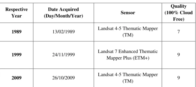
This research is dependent on secondary data. To prepare the base maps for analysis purpose and applying the different methods to achieve the research objectives, Landsat satellite images (1989, 1999 and 2009) have been collected from the official website of U.S. Geological Survey (USGS). Table 2.1 shows the details of the Landsat satellite images used for analysis.
Table 2.1: Details of Landsat Satellite Images
Respective Year
Date Acquired
(Day/Month/Year) Sensor
Quality (100% Cloud
Free)
1989 13/02/1989 Landsat 4-5 Thematic Mapper
(TM) 7
1999 24/11/1999 Landsat 7 Enhanced Thematic
Mapper Plus (ETM+) 9
2009 26/10/2009 Landsat 4-5 Thematic Mapper
(TM) 9
Source: U.S. Geological Survey, 2010 [21]
Landsat Path 137 Row 44 covers the whole study area. Map Projection of the collected satellite images is Universal Transverse Mercator (UTM) within Zone 46 N– Datum World Geodetic System (WGS) 84 and the pixel size is 30 meters [21].
Figure 2.2 illustrates the location of DCC on the Landsat satellite images for different years. The surroundings of DCC have also been included within the study area for predicting the future land cover changes.
Chapter 2 17 Figure 2.2: Dhaka City Corporation and its Surroundings
Chapter 2 18 2.3.3.2 Reference Data
For the purpose of ground-truthing/ referencing, several base maps of Dhaka City (for the year of 1987, 1995 and 2001) have been collected from the Survey of Bangladesh (SoB). Again, for comparing the images some other reference satellite images (IRS image of 1996 and Landsat satellite image of 2003) have been collected from the Department of Urban and Regional Planning, Bangladesh University of Engineering and Technology (BUET), Dhaka, Bangladesh. The land use maps of all the wards of DCC (2008) have been collected from DCC and Rajdhani Unnayan Kartripakkha (RAJUK) or Capital City Planning and Development Authority. Google Earth is another option to get some ideas about the recent land cover pattern of Dhaka city. These reference data have been used for training site selection and preparing land cover maps.
The collected base maps are attached in Appendix B.
2.3.3.3 Literature Review
To understand the concept and methods of urban land cover change pattern analysis and prediction, and collect some necessary information; many papers and documents have been collected. In this regard various journal papers, reports, conference papers and dissertations have been overviewed.
2.3.4 Base Map Preparation and Accuracy Assessment
For image classification purpose, a fisher supervised classification method has been used. Then after achieving satisfactory accuracy results, the base maps have been finalized. Details of the procedures of base map preparation and accuracy assessment have been described in Chapter 3.
2.3.5 Change Detection Analysis
The change detection of urban land cover types have been analyzed using different available techniques. Details can be found in Chapter 4.
2.3.6 Model Calibration/ Simulation
Chapter 2 19 2.3.7 Model Validation and Selection
At first the classified base land cover images of Dhaka city of 1989 and 1999 have been used to predict the land cover map of 2009 using the selected three methods. Then map comparison techniques have been applied between the predicted and classified land cover map of 2009. This is known as model validation. Out of the three methods implemented, the most suitable model for this particular research has been chosen based the kappa statistics. Model validation and selection techniques and the results are described in detail in Chapter 8.
2.3.8 Future Prediction
The land cover map of 2019 of Dhaka city has been predicted using the method obtained from model selection process. The simulation process and the analysis of the predicted map (2019) have been elaborated in Chapter 09.
2.3.9 Directions for Future Planning
A few recommendations have been devised for future planning of Dhaka city, based on the results found from this research. This can be found in Chapter 10.
2.3.10 Report Writing
After getting all relevant data and information related to the concerned aspects, data analysis and the subsequent interpretations; all these are presented in this thesis report.
2.4 Tools Used for this Research
Different software programs have been used for conducting this research. These are:
Image Classification and Model Simulation: „IDRISI 16: The Taiga Edition‟.
Accuracy Assessment: „ERDAS IMAGINE 9.1‟.
Change Detection Analysis: „Fragstats 3.3‟.
Model Validation: „The Map Comparison Kit: version 3.2.0‟.
Map Projections and Preparation: „ArcGIS 9.3.1 Desktop‟.
Chapter 3 20
Chapter 3
Base Map Preparation and Accuracy Assessment
This chapter deals with explaining the procedure of preparing the base maps for analysis and the accuracy assessment of those maps.
The collected Landsat satellite images (1989, 1999 and 2009) have been used for preparing the base maps for land cover change detection and future prediction. The basic steps for preparing the base maps are as follows:
3.1 Image Enhancement
Image enhancement is a kind of image modification that enables the capabilities of human vision to identify and select regions of interests [35]. Composite generation technique has been performed for this particular research.
3.2 Composite Generation
Landsat TM records 7 spectral bands. For visual purpose any 3 bands are combined that are acting a False Color Composite (FCC). Figure 3.1 shows several composites using different band combinations from the same TM images [36].
Figure 3.1: Composites Using Different Band Combinations [36]
Using the basic colours red, green and blue (RGB) it is possible to prepare different FCC images [37]. These FCC images are useful to distinguish between different cover types or ground objects like buildings, roads, and vegetation.
Chapter 3 22 The study area is selected by choosing the same geographic position of all 7 bands for the same time period. This helps to maintain the same number of rows and column. The properties of each image are described in Table 3.1.
3.3 Image Classification
Image classification refers to grouping image pixels into categories or classes to produce a thematic representation [39]. Image classification comprehends various operations that can be applied to photographic or image data. These include image restoration, image pre-processing, enhancement, compression, spatial filtering, and pattern recognition and so on [39]. There are two basic methods of image classification: supervised and unsupervised [37]. Supervised classification relies on the priori knowledge of the study area [39]. Therefore, for this research, a supervised classification method has been used.
Supervised classification can be defined as: “A procedure for identifying spectrally similar areas on an image by identifying ‘training’ sites of known targets and then extrapolating those spectral signatures to other areas of unknown targets” [39].
In case of supervised classification, the user develops statistical description for various known land cover types that is called signature development. Then a procedure is used to identify the similar pixels/signature for different land cover types for the whole image. The steps that are followed for this supervised classification are as follows:
3.3.1 Training Site Development
Chapter 3 23 Table 3.1: Properties of the Processed Raster Images for Analysis
Table 3.2: Details of the Land Cover Types Image Characteristic Description
File Format Raster
File Type Binary
Data Type Byte
Columns 650
Rows 762
Reference System UTM-46 North
Reference Unit Meter
Datum WGS 84
Minimum X 224445
Maximum X 243945
Minimum Y 2621445
Maximum Y 2644305
X Resolution 30
Y Resolution 30
Land Cover Type Description
Builtup Area All residential, commercial and industrial areas, villages, settlements and transportation infrastructure.
Water Body River, permanent open water, lakes, ponds, canals and reservoirs.
Vegetation
Trees, shrub lands and semi natural vegetation: deciduous, coniferous, and mixed forest, palms, orchard, herbs, climbers, gardens, inner-city recreational areas, parks and playgrounds, grassland and vegetable lands.
Low Land
Permanent and seasonal wetlands, low-lying areas, marshy land, rills and gully, swamps, mudflats, all cultivated areas including urban agriculture; crop fields and rice-paddies.
Fallow Land
Chapter 3 24 3.3.2 Signature Development
This is the stage of creating the spectral signature for each type of land cover. This is done by analyzing the pixels of the training sites [36]. When the digitization of training sites is finished, the statistical characterizations of each land cover class are needed. These are called signatures.
Signatures are developed incorporating the vector files containing training sites and the bands used for analysis. These signature files contain statistical information about the reflectance values of the pixels of the training sites for each land cover type [36].
3.3.3 Classification
After developing signature files for all land cover classes the next step is to classify the images based on these signature files. This can be done by two ways: hard or soft classifiers [37]. These are kind of statistical techniques to classify the whole image pixel by pixel based on each known type particular signature [36].
In case of hard classifications, each pixel is assigned in a way that has the most similar signature for a particular land cover type. On the other hand, soft classifications take into consideration the degree of membership of the pixel in all classes [37].
For this research, a hard classifier called „Fisher Classifier‟ has been chosen. Fisher classifier uses the concept of the linear discrimination analysis [36]. Fisher Classifier performs well when there are very few areas of unknown classes and when the training sites are representative of their informational classes [37]. This is why fisher classifier is appropriate for this particular research, because most areas for the classes are known.
3.3.4 Generalization
After image classification, sometimes many isolated pixels may be found [37]. These isolated pixels may belong to one or more classes that differ from surrounding pixels. Therefore it is necessary to generalize the image and remove the isolated pixels.
Chapter 3 25 Therefore, a 3×3 mode filter has been applied to generalize the fisher classified land cover images. This post-processing operation replaces the isolated pixels to the most common neighbouring class. Finally the generalized image is reclassified to produce the final version of land cover maps for different years (Figure 3.3).
Chapter 3 26
3.4 Accuracy Assessment
The final stage of image classification process is accuracy assessment. Accuracy Assessment is a kind of process to compare the classification with ground truth or other data. It allows evaluating a classified image file [36].
It is not typical to ground truth each and every pixel of the classified image. Therefore some reference pixels are generated. Reference pixels are points on the classified image. Each point of reference pixels represents specific geographic coordinate of the image. These reference pixels are randomly selected [40].
The randomly selected points within the classified image list two sets of class. The first set of class values represents the actual land cover type. The second set of class values are known as reference values. These reference values are input by the researcher that is based on ground truth data [41].
The ground truthing of reference values are possible through field visit, comparing base maps, aerial photos, previously tested maps or other data [41].
The number of reference pixels is an important issue for accuracy assessment. It has been proved that more than 250 reference pixels (± 5%) are needed to estimate the mean accuracy of classification [40].
Therefore 250 reference pixels have been generated for each classification image for this research to perform accuracy assessment.
There is a common tendency while selecting the reference pixels by the analysts. The researchers often select the same pixels as reference pixels for testing the classification that had already been used for training samples [40]. This creates kind of biasness.
This is why the reference pixels are normally selected randomly to eliminate this kind of impartiality [40].
Therefore for this research, the reference pixels have been selected using stratified random distribution process.
Chapter 3 27 3.4.1 Assessment Procedure
The collected base maps (Appendix B) have been used to find the land cover types of the reference points. Figure 3.4 and Table 3.3 (not real, just an example to show how the mechanism works within the overall procedure) show how the land cover types for the randomly selected points are chosen.
Here (Figure 3.4) the representation is like; 1= Builtup Area, 2= Water Body, 3= Vegetation, 4= Low Land and 5= Fallow Land.
Figure 3.4: Random Points Cell Listing
Figure 3.4 shows the process of selecting the stratified random points for different land cover types within a specific cell.
To select the random reference pixels, a 3×3 window has been selected for cell listing. Then the mid-value of each cell is generated as random point (Figure 3.4). The numbers in parenthesis are the chosen land cover type values for each cell.
This is how 250 random points showing class values have been selected from 250 cells. Cell 1 (5)
5 5 5
5 5 5
5 5 5
Cell 2 (2)
1 2 2
2 2 1
2 2 2
Cell 3 (4)
5 5 4
4 4 4
4 5 4
Cell 4 (1)
1 1 3
3 1 3
1 1 1
Cell 5 (1)
4 4 4
1 1 1
1 1 1
Cell 6 (5)
2 5 5
2 5 5
2 5 5
Cell 7 (3)
1 1 3
3 3 3
4 3 3
Cell 8 (1)
1 1 1
5 1 1
Chapter 3 28 Table 3.3: Accuracy Assessment Cell Array
Table 3.3 illustrates the cell array for accuracy assessment. The right-most columns respectively represent the class values and reference values. The class values are generated from as per the rules mentioned in Figure 3.4. The reference values, cross-checked from base maps, are input from the researcher.
Moreover, this figure shows the point IDs‟ and the geographic coordinates (X and Y
values) for each random point. At the end, 250 land cover class and reference values have been randomly selected for the base years of 1989, 1999 and 2009.
Figure 3.5 shows the randomly selected 250 points for each base year.
From the accuracy assessment cell array, three types of reports are generated [41]. These are:
a) Error Matrix: it compares the reference points to the classified points in a c×c matrix, where c is the number of land cover classes.
b) Accuracy Totals: it calculates statistics of the percentages of accuracy that is based on the error matrix and
c) Kappa Coefficient.
Details of the basic terms used for accuracy assessment have been explained in Appendix C. Moreover, the related tables of the accuracy reports for different time periods have been stated from Table C 4 to C 12 (Appendix C).
Point Name ‘X’ Co-ordinate ‘Y’ Co-ordinate Class Reference Result
1 ID#1 232230.00 2643810.00 5 5 Correct
2 ID#2 230220.00 2628480.00 2 1 Incorrect
3 ID#3 232560.00 2630907.00 4 4 Correct
4 ID#4 225180.00 2868000.00 1 1 Correct
5 ID#5 225270.00 2634120.00 1 1 Correct
6 ID#6 239220.00 2643210.00 5 4 Incorrect
7 ID#7 243870.00 2637990.00 3 3 Correct
Chapter 3 30 3.4.2 Results and Discussion
The assessment of classification accuracy of the land cover maps (1989, 1999 and 2009) has been carried out using error matrices (Table C 4, C 7 and C 10).
User‟s accuracy measures the proportion of each land cover class which is correct. On the other hand, producer‟s accuracy measures the proportion of the land base which is correctly classified. Producer‟s and User‟s accuracy are also found consistently high ranging from 71%-100% (Table C 5, C 8 and C 11) for all the years. Therefore, higher
values of producer‟s and user‟s accuracy indicate that the prepared base maps are quite
good enough for further analysis.
Overall accuracy takes no account of source of error. Kappa coefficient is a measure of the proportional (or percentage) improvement by the classifier over a purely random assignment to classes. The overall accuracies for 1989, 1999 and 2009 are found 85.20%, 86.80% and 91.60% respectively, with Kappa statistics of 0.8054, 0.8294 and 0.8592 (Appendix C). The conditional kappa values for each category for different years are also found higher (Table C 6, C 9 and C 12).
It means few misclassifications have been observed in the classified land cover maps of Dhaka city. This may be because of the same spectral characteristics of some land cover types. For example, in case of 1989 base map, certain built-up areas were misclassified as fallow land. Again, in most cases it was really difficult to separate water bodies and low/cultivable lands categories. The reasons may be the seasonal variations of the satellite images for different years and the similar spectral properties of land covers in some cases.
Moreover, less image spectral resolution has directed to spectral mixing of different land cover types. This has caused spectral confusions among the cover types. It is also important to mention that the images of 1999 and 2009 represent winter season while the image of 1989 represents spring season. Therefore other seasonal images can be important evaluating the land cover change pattern of this kind of highly dynamic urban environment like Dhaka.
Chapter 4 31
Chapter 4
Land Cover Change Detection Analysis
The different techniques and spatial metrics that have been implemented for change detection analysis are described in this chapter.
4.1 Change Detection
Urban area is highly dynamic. Numerous factors put impact on the growth or changing pattern for a particular city. Therefore, understanding the urban dynamics is a complex task while planning for a planned and sustainable urban development [48]. To predict the future change of highly dynamic urban areas like Dhaka city, it is necessary to assess and monitor the urban land cover change on a regular basis. In remote sensing, ‘Change Detection’ is defined as the process of determining and monitoring the changes in the land cover types in different time periods. It provides the quantitative analysis of the spatial distribution in the area of interest [48]. Change detection is important because it helps the researcher to understand and monitor the land cover change pattern (e.g. urbanization, deforestation, agricultural land management) within the study area.
Change detection can be divided into two major groups: pre-classification and post-classification methods. A number of approaches like image differencing, image rationing, vegetation index differencing (NDVI), principal component analysis, artificial networks, fuzzy sets, object-oriented methods, image regression etc; have been applied in numerous studies to determine the spatial extent of land cover types [48]. Among these methods, post-classification is the most common and suitable method for detecting land cover change analysis [30]. The accuracy of change detection is dependent on the accuracy of each land cover type. Therefore, performing change detection analysis should be done after land cover classification [30]. Considering all these things post-classification method has method has been applied for this research.
4.2 Terminologies
Chapter 4 32 4.3 Analysis and Interpretation of the Change Detection Techniques
Class-level metrics are integrated over all the patches of a given type (class) [50]. For this research purpose, class-level metrics have been used. There are five broad categories of land cover types in this study. Therefore, the spatial metrics values for all these types have been generated for all the base years (1989, 1999 and 2009). The raw values in tabular format are attached in Appendix E. In this section, the interpretation of the generated values of selected spatial metrics and other techniques has been discussed.
4.3.1 Number of Patches and Largest Patch Index
Figure 4.1: Number of Patches and Largest Patch Index
The numbers of patches, urban blocks in this case, of builtup area and fallow land types have increased over time. Again the decrease of water body and vegetation is prominent (Figure 4.1). This reveals the gradual development of urban infrastructures converting water bodies, vegetation and low lands.
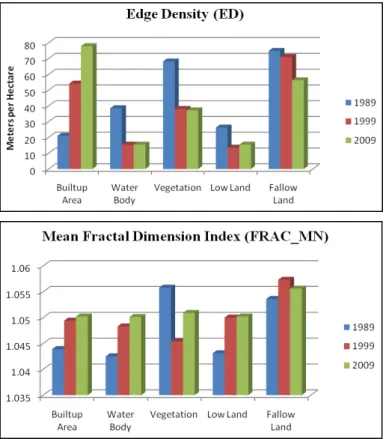
Chapter 4 33 4.3.2 Edge Density and Mean Fractal Dimension Index
Edge density (ED) of builtup area is increasing, while ED of fallow land, vegetation and water body cover types are decreasing (Figure 4.3). The total length of the edge of the land cover patches (urban patch) increases with an increase in the land use fragmentation and development of continuous urban features [48]. Therefore, this gradual increment in builtup area proves an increase in the total length of the edge of the urban patches.
Figure 4.2: Edge Density and Mean Fractal Dimension Index
A FRAC_MN value greater than 1 for a 2-dimensional patch indicates a departure from Euclidean geometry (i.e., an increase in shape complexity). FRAC_MN approaches 1 for shapes with very simple perimeters such as squares, and approaches 2 for shapes with highly convoluted, plane-filling perimeters [50].
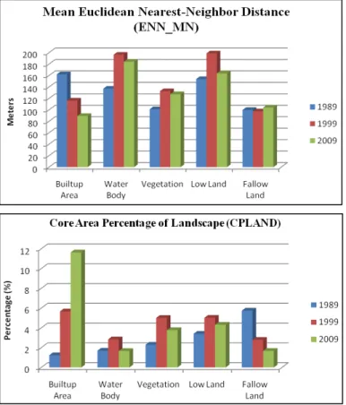
Chapter 4 34 4.3.3 Mean Euclidean Nearest-Neighbour Distance and CPLAND
Mean Euclidean Nearest-Neighbour Distance (ENN_MN) approaches 0 as the distance to the nearest neighbour decreases. It is perhaps the simplest measure of patch context and has been used extensively to quantify patch isolation [50]. ENN_MN of builtup area land cover type is decreasing over time (Figure 4.4). This proves that the urban patches of builtup area type are getting closer to each other. It means the urban areas are getting clumsy indicating absence of proper planning.
Figure 4.3: ENN_MN and CPLAND
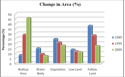
Chapter 4 35 4.3.4 Change in Area
There are three possible change detection analyses over time for this research. These are change between 1989 and 1999, 1999-2009 and 1989-2009. The summaries of land cover classification statistics (1989-1999) have been attached in Appendix F.
Figure 4.4: Land Cover Change in Area (Percentage)
It is clear that over the years (1989 to 2009) builtup area has increased in huge percentage (from 8.4% to 46%). It is also noteworthy that fallow has decreased in good rate (from 38% to 17%). Other land cover types have decreased in a very small amount (Figure 4.4).
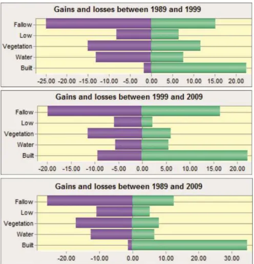
4.3.5 Gains and Losses by Category
Figure 4.5 illustrates that builtup area has increased over the years while there is slight loss in this category. It means some parts of the previously existed builtup areas have converted to some other land cover classes, while vast new area has transformed into builtup area from other classes.
Gains in builtup area are evident in all three combinations. Again fallow land cover type is decreasing in large percentage in all the years. The changes (in terms of gains and losses) in other land cover types are almost the same or not influencing.
Chapter 4 36 Figure 4.5: Gains and Losses of Land Covers by Category (Unit: % of Area)
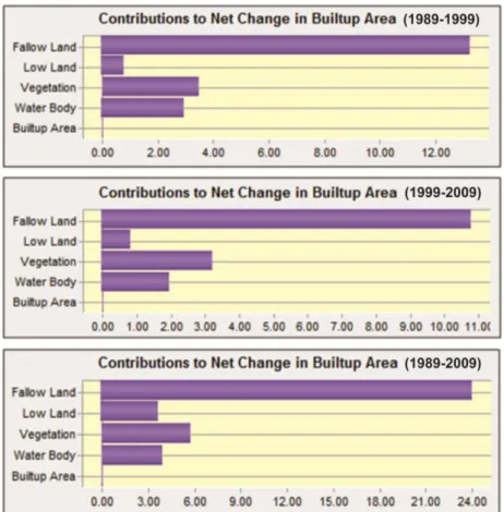
4.3.6 Contributors to Net Change Experienced by Builtup Area
Figure 4.6 illustrates which land cover type is contributing more to net change in built-up area. It is found that fallow land is contributing most converting towards builtbuilt-up area followed by water body and vegetation.
4.3.7 Transition to Builtup Area
Figure 4.7 shows which areas from other land cover types have been converted to built-up areas. The dominance of fallow land (orange color) is clear here which justifies the explanation of Figure 4.6.
Chapter 4 37 Figure 4.6: Contributors to Net Change Experienced by Builtup Area (Unit: % of Area)