www.atmos-chem-phys.net/14/10963/2014/ doi:10.5194/acp-14-10963-2014
© Author(s) 2014. CC Attribution 3.0 License.
TNO-MACC_II emission inventory; a multi-year (2003–2009)
consistent high-resolution European emission inventory for air
quality modelling
J. J. P. Kuenen, A. J. H. Visschedijk, M. Jozwicka, and H. A. C. Denier van der Gon TNO, Department of Climate, Air and Sustainability, Utrecht, the Netherlands
Correspondence to:J. J. P. Kuenen ([email protected])
Received: 20 December 2013 – Published in Atmos. Chem. Phys. Discuss.: 5 March 2014 Revised: 29 August 2014 – Accepted: 1 September 2014 – Published: 17 October 2014
Abstract. Emissions to air are reported by countries to EMEP. The emissions data are used for country compliance checking with EU emission ceilings and associated emission reductions. The emissions data are also necessary as input for air quality modelling. The quality of these “official” emis-sions varies across Europe.
As alternative to these official emissions, a spatially explicit high-resolution emission inventory (7×7 km) for
UNECE-Europe for all years between 2003 and 2009 for the main air pollutants was made. The primary goal was to sup-ply air quality modellers with the input they need. The inven-tory was constructed by using the reported emission national totals by sector where the quality is sufficient. The reported data were analysed by sector in detail, and completed with alternative emission estimates as needed. This resulted in a complete emission inventory for all countries.
For particulate matter, for each source emissions have been split in coarse and fine particulate matter, and further disag-gregated to EC, OC, SO4, Na and other minerals using
frac-tions based on the literature. Doing this at the most detailed sectoral level in the database implies that a consistent set was obtained across Europe. This allows better comparisons with observational data which can, through feedback, help to fur-ther identify uncertain sources and/or support emission in-ventory improvements for this highly uncertain pollutant.
The resulting emission data set was spatially distributed consistently across all countries by using proxy parameters. Point sources were spatially distributed using the specific lo-cation of the point source. The spatial distribution for the point sources was made year-specific.
The TNO-MACC_II is an update of the TNO-MACC emission data set. Major updates included the time extension
towards 2009, use of the latest available reported data (in-cluding updates and corrections made until early 2012) and updates in distribution maps.
1 Introduction
Over the last decades, environmental problems such as acid-ification, eutrophication, air pollution and climate change have caused significant adverse impacts on human health and vegetation (EEA, 2010). Only part of the air pollution emis-sion reductions set by the 2010 National Emisemis-sion Ceilings have been achieved (EEA, 2012a), therefore transboundary air pollution remains a problem (EEA, 2010). All these en-vironmental problems are directly related to the emissions of substances to air. Reliable emission inventories are a pre-requisite to understand these environmental issues and to de-velop effective mitigation options.
For a good understanding of environmental problems, not only the magnitude of the sources but also their location is important. The spatially distributed emissions need to cover the complete domain, and describe the emissions in a con-sistent way, i.e. in all countries the same sources should be included, and these sources should be assessed as accurately and consistently as possible.
approach has been taken also by many countries that pro-duce annual emission inventories for greenhouse gases and air pollutants, since they have to report their emissions under the various international treaties. Over time, as experience and expertise has increased, the number, substances covered and quality of these inventories has significantly improved (EMEP, 2013). These in-country systems take into account all country-specific information and national legislation and are therefore capable of providing a more accurate estimate of the emissions compared to a regional or global emission inventory.
When using regional chemical-transport modelling in pol-icy studies, the use of these official inventories is often re-quired. However, the official emissions still contain a num-ber of gaps and shortcomings, e.g. not all countries report according to the requirements (EMEP, 2013). This paper presents a complete, consistent and spatially distributed in-ventory, which has used the official reported emissions as ba-sis where possible. This makes this inventory suitable for ap-plication in policy-related modelling and impact studies for air pollution. The TNO_MACC-II inventory is the successor of the widely used GEMS inventory for 2000 (Visschedijk et al., 2007) and the TNO_MACC inventory for the years 2003–2007 (Kuenen et al., 2011; Pouliot et al., 2012).
2 Methodology 2.1 Emission estimates
The Convention for Long-Range Transboundary Air Pol-lution (CLRTAP; http://www.unece.org/env/lrtap/) requires countries to report their emissions. Fifty-one countries in Eu-rope and North America, including the EU as a whole, have to annually submit their emissions of air pollutants for the latest year and all historic years to EMEP (the co-operative programme for the monitoring and evaluation of long-range transmission of air pollutants in Europe). The reporting fol-lows well-defined guidelines and asks countries to complete a pre-defined template with emissions by year, pollutant and sector (defined by the Nomenclature for Reporting; NFR). Countries are encouraged to set up their own inventory sys-tem and choose the best methodologies for emission esti-mation which fit their national situation. For larger sources, Parties have to use more advanced methodologies, with cific emission factors for each technology. When no spe-cific national methodology is available, the EMEP/EEA Air Pollutant Emission Inventory Guidebook (EEA, 2013) pro-vides default guidance on how to estimate emissions for each sector. The official submitted data for all countries are col-lected by the Centre for Emission Inventories and Projections (http://www.ceip.at/) and made available online. Because of the more detailed methodologies included in most invento-ries and the national focus of each of the inventoinvento-ries, the re-ported emissions often provide the most accurate estimate for
Table 1.Explanation of the SNAP source categories (SNAP 3 and SNAP 4 are merged to SNAP 34).
SNAP Sector name
1 Energy industries 2 Non-industrial combustion 34 Industry (combustion+processes) 5 Extraction and distribution of fossil fuels 6 Product use
7 Road transport
8 Non-road transport and other mobile sources 9 Waste treatment
10 Agriculture
a country. However, in many cases gaps and errors do exist in the reported emission data. In particular, the consistency in emissions reporting for consecutive years is problematic.
In order to assess the quality of the reported emissions, we have downloaded the data from CEIP (CEIP, 2012) for CO, NOx, SO2, NMVOC, NH3, PM10 and PM2.5and from
EEA (EEA, 2012b) for CH4for all countries for the period
2003–2009. Before analysing the data in detail, we have first aggregated the NFR sectors to 43 individual sectors (link table available from the Supplement, Excel file number 1). These 43 sectors were defined based on the SNAP (Selected Nomenclature for Air Pollution) at level 1 with one addi-tional level of detail for most sectors. Industrial combus-tion (SNAP 3) and industrial process emissions (SNAP 4) have been aggregated to a new defined SNAP 34. This was done because there is often confusion between combustion and process emissions for a particular plant or facility, partly because countries may have slightly different definitions on where to draw the line or how to report. In an overarching Eu-ropean inventory this problem is effectively solved by merg-ing both categories. An explanation of the SNAP source cat-egories as used in this study is given in Table 1.
For this data set we have analysed the time series between 2003 and 2009 in detail. Where the time series or the sector split of the total country emissions was not understandable (e.g. unexplainable jumps in the trend, multiple years of data missing, not understandable sector splits), the data were dis-carded.
intervals. To obtain emissions for the years in between, lin-ear interpolation was used where necessary.
The GAINS model does not calculate emissions of CO. In the case that no country reported CO emissions of suffi-cient quality were available the CO emissions are gap-filled using a bottom-up emission inventory which has been de-veloped at TNO for the year 2005. Like the GAINS model or the EDGAR inventory (JRC, 2011), this bottom-up inventory is built up using activities such as the energy statistics and industrial production figures as the baseline in combination with the most appropriate emission factors. In the transport sector, this means that data from the TREMOVE model (De Ceuster et al., 2005) were used to disaggregate the energy use to detailed vehicle classes technologies for each country. These were combined with state-of-the-art emission factors for each technology for road transport (Ntziachristos et al., 2009) to calculate the emissions. When less detail was avail-able for certain source categories, technology-specific emis-sion factors were applied to groups of countries with a similar technology level. Since this bottom-up inventory was orig-inally only developed for the year 2005, emissions for the other years were estimated by scaling this inventory. Scal-ing factors for the different years were calculated from the EDGAR emission inventory v4.2 (JRC, 2011), which pro-vides sector-specific annual emission estimates for CO for each country in the world.
For the countries Armenia, Azerbaijan and Georgia, nei-ther reported nor GAINS emission data were available. Therefore, EDGAR (JRC, 2011) data were used at SNAP level 1 (see Table 1) for these countries for all pollutants and all years. These were disaggregated to the same subcate-gories as the other countries by using the relative contribution of each subsector to the SNAP level 1 sector for Turkey (for each pollutant and each year) as a blueprint.
To illustrate in more detail the extent to which each data source has been used, the Supplement (Excel file number 2) includes a table which shows the main source of the emis-sions that was used, per country per pollutant. However, for underlying sectors the choice of which emission source to use may have been updated based on the checks that were performed. In the final data set, the share of reported data in the total emissions varies between 40 % (for PM) and 70 % (for NH3). In geographical terms, reported emissions were
the primary data source for most EU Member States and EFTA countries, while for many former Soviet Union coun-tries and some Balkan councoun-tries the use of GAINS or other alternative data sources was necessary. The Excel file num-ber 2 in the Supplement also contains a full overview of the choices made per country, pollutant and sector.
2.1.1 Consistency between countries and across years Emission data for certain years may be missing (Figs. 1 and 2, left panel), and countries may use different classifica-tions or differ in what sources they report. To improve
con-0 5 10 15 20 25 30 35
2003 2004 2005 2006 2007 2008 2009
E
m
is
si
o
n
(
kt
o
n
) LVA, SNAP 34
CZE, SNAP 10 HUN, SNAP 2 BGR, SNAP 2 RUS, SNAP 2
Figure 1.Observed trends in PM10reported emissions for selected countries and SNAP level 1 source categories (source: CEIP, 2012).
sistency between countries, a number of updates have been made to the resulting data set which mainly affected the re-ported emissions data.
– Emissions of NOxand NMVOC from agriculture have
been removed for all countries, since reporting of this source is found to be very inconsistent between coun-tries. For NOx, 3/4 of the removed NOx(approximately
150 kt annually) was reported by Germany as emissions from biological N fixation and crop residues, which is not reported by other countries. There is a risk that some of the other countries reported emissions from agricul-tural machinery in SNAP 10 instead of SNAP 8 which is then “lost”.
– Emission estimates for national shipping were found to be very inconsistent between countries, partly due to different definitions for the various sectors (allocation issue). To avoid inconsistencies and double counted or missing emissions to the extent possible, all national shipping including international inland shipping emis-sions have been replaced with TNO estimates, which distinguish inland shipping and coastal shipping as sep-arate sources. Especially with international inland nav-igation, countries may treat this differently in their in-ventories.
– Estimates for emissions from agricultural waste burn-ing have been replaced by GAINS emissions because only few countries reported emissions from this source, while emissions are significant especially for PM. This adds about 350 kt PM10per year to our inventory, where
the sum of the country values adds up only to 16 kt (in 2009).
– For particulate matter, numerous cases were found where reported PM2.5 exceeded reported PM10. These
have been corrected by increasing PM10 emissions to
PM2.5levels. This implies that in such cases the coarse
0 0.2 0.4 0.6 0.8 1 1.2 1.4
2003 2004 2005 2006 2007 2008 2009
No rm al is ed emi ss io n (20 09 =1)
Reported emissions trends
NOX EU15,CHE,NOR NOX EU13 NOX Other countries PM10 EU15,CHE,NOR PM10 EU13 PM10 Other countries
0 0.2 0.4 0.6 0.8 1 1.2 1.4
2003 2004 2005 2006 2007 2008 2009
No rm al is ed emi ss io n (20 09 =1)
Reported emissions trends
NOX EU15,CHE,NOR NOX EU13 NOX Other countries PM10 EU15,CHE,NOR PM10 EU13 PM10 Other countries
0 0.2 0.4 0.6 0.8 1 1.2 1.4
2003 2004 2005 2006 2007 2008 2009
No rmal is e d e mi ss io n ( 2009= 1)
TNO_MACC-II emissions trends
NOX EU15,CHE,NOR NOX EU13 NOX Other countries PM10 EU15,CHE,NOR PM10 EU13 PM10 Other countries
Figure 2.Trends in reported emissions (left panel) and TNO_MACC-II (right panel) normalized to 2009=1.
Table 2.Sulfur content assumed in the fuel for the calculation of in-port emissions (in %).
Year North Sea Baltic Sea Other EU(27) Non-EU(27)
2005 1.335 1.335 1.335 1.335
2006 1.335 1.095 1.335 1.335
2007 1.305 0.975 1.335 1.335
2008 0.975 0.975 1.335 1.335
2009 0.975 0.975 1.335 1.335
2010 0.1 0.1 0.1 1.335
– Emissions from international shipping have been taken from CEIP (2012) for all years and pollutants.
– NMVOC, SO2, NOx, CO and PM shipping emissions
for the 43 largest North Sea ports (including oil ter-minals) were additionally included. For the year 2009, these data were taken from MARIN (Cotteleer and Van der Tak, 2009). For SO2 and PM a strong decreasing
emission trend for the period 2005 to 2010 is expected as a result of implementation of European sulfur reduc-tion policies (EC, 2011). The assumed average sulfur contents in marine fuel used for the calculation of in-port emissions is presented in Table 2. SO2 and PM
emissions have been scaled accordingly from the 2009 emission data. Emissions of other substances are as-sumed to be constant at 2009 level for the 2003–2009 period. From the MARIN emission data, implied emis-sion factors based on port turnover capacity were de-rived and applied to the 1200 other ports in Europe, for which capacity data was taken from the PAREST emis-sion database (Denier van der Gon et al., 2010). Based on Google Maps and visual identification of port activ-ities the 1/8×1/16◦cells occupied by the 43 MARIN ports have been manually selected (e.g. the Port of Rot-terdam occupies seven of such cells). Geographical dis-tribution of emission within cells associated with a cer-tain port is assumed to be uniform. The location of the centre point of the 1200 other ports in Europe has been
taken from the PAREST emission database (Denier van der Gon et al., 2010).
To be suitable as model input the emissions need to be distributed on a grid (see Sect. 2.3), for which a more de-tailed sectoral breakdown is needed to allow for a different spatial distribution of different subsectors and fuels under-lying the 43 sectors. Therefore, emissions have been dis-aggregated using the more detailed data available from the GAINS model and the TNO bottom-up inventory (for CO). For power plants, residential combustion and road transport (exhaust) the emissions are disaggregated to main fuel type (coal, gas, solid biomass, waste or light, medium or heavy liquid fuels). For some other sectors such as the iron and steel and non-ferrous metal industries, emissions are disag-gregated to subsectors. An overview of the disagdisag-gregated sectoral classification is given in the Supplement (Excel file number 3).
2.2 Particulate matter composition
For particulate matter, the emissions have been further dis-aggregated from PM2.5and PM10 to various components in
the coarse and fine mode. To calculate this PM split, more detailed sectoral information is needed, for example the fuel type used in combustion installations and the type of instal-lation. Therefore, the emission data are first disaggregated to GAINS sector and activity combinations (more than 200 categories).
For each GAINS category, a fractional split between 5 PM components (EC, OC, SO4, Na and other minerals) was made
year 2005 (Visschedijk et al., 2007). This inventory involved creating “best estimates” per GAINS sector and activity com-bination for EC and OC fractions in PM, based on literature data and three earlier EC and OC emission inventories.
Particle-bound sulfate is mostly emitted through the com-bustion of high-sulfur fuels such as coal and residual fuel oil. In the LOTOS-EUROS model (Schaap et al., 2008) it is esti-mated that around 2 % of the sulfur is emitted in the form of particles. When particle mass is calculated based on the SO2
emissions using this estimation, the fraction of sulfur emit-ted in the form of particles ranges from 0.1 % for gasoline and diesel combustion in road transport to 10–20 % for coal and residual fuel oil combustion in energy and manufacturing industries and in shipping.
The sodium fraction is relatively unimportant to the total PM but may be useful when looking at base cation deposi-tion. The sodium content is based on reported sodium content for 40 PM sources calculated in Van Loon et al. (2005).
The fraction “Other minerals” contains other non-carbonaceous particles and is calculated as the remaining fraction after the other fractions have been calculated.
The fractions per GAINS category have been applied to the emissions of coarse PM (PM10–PM2.5) and fine PM
(PM2.5) for each GAINS category, and subsequently been
ag-gregated to the 77 source categories which are used as input to the spatial distribution.
EC and OC country total emissions (for both fine and coarse mode) are given for all years in the Supplement, Excel file number 5.
2.3 Spatial distribution
The final step in the inventory was the distribution of the complete emission data set across the European emission do-main at 0.125◦×0.0625◦ longitude–latitude resolution. For
each of the 77 source categories for which emissions are available, one or more proxies were identified. These proxies provide the mapping of the emissions of a certain pollutant to the grid for a given sector and year. For each country, pollu-tant, sector and year the most appropriate proxy was chosen in a selection table. An overview of all the proxies used per sector is given in the Supplement (Excel file number 3).
For point sources, we have made use of the E-PRTR database (http://prtr.ec.europa.eu/) which provides informa-tion on the locainforma-tion (longitude, latitude) and emissions of major facilities in Europe. E-PRTR data were available on an annual basis from 2007 onwards, while data from the years 2001 and 2004 were available from its predecessor EPER (EC, 1996). For the intermediate years, data from the closest year available were used. Since the EPER and E-PRTR data only contain emissions from facilities above a certain thresh-old, using these data to distribute total emissions for a certain sector can only be done for those sectors comprised of large facilities, e.g. the cement and aluminium industries. Further-more, a judgement has been made on the quality of the data
before actually using them. For example, there are multi-ple facilities where the geographical location points to the administrative location (e.g. company headquarters) rather than the location where the actual emissions occur. For the other point sources, and also those in countries which are not covered by E-PRTR, TNO’s own point source database (de-scribed in more detail in Denier van der Gon et al., 2010) was used as a proxy for the distribution of these point source emissions.
For non-point sources (e.g. residential combustion, trans-port sectors, agriculture), proxies were selected to distribute country total emissions over the grid. These proxies include (among others) total, rural and urban population, arable land, TRANSTOOLS road network (JRC, 2005). The proxies for the area sources were assumed to be static in time, e.g. changes in the population density are not taken into account. Most proxy maps were taken from Denier van der Gon et al. (2010) but a number of modifications and improvements have been made. A new population map for the year 2005 has been implemented at high resolution, and a special proxy has been developed for the distribution of residential wood combustion. The latter takes into account both the population density, but also the proximity to wood. Despite this modifi-cation for the distribution of residential wood combustion, an overallocation of the emissions in urbanized centres may well be present in the spatial distribution. This has previously been described by Timmermans et al. (2013). However, a universal, representative and well-documented approach that justifies a modification of the spatial distribution between ur-ban and rural areas for Europe does not exist at this moment. For the actual calculation of the emissions grids, a SQL server system has been set up which performs all the calcu-lations. Emissions that could not be distributed (e.g. because the proxy was not available for that specific country) are by default distributed using either total population, rural popu-lation or arable land. In a last step the gridded emissions are aggregated to SNAP level 1, primarily to reduce the size of the output emission grid file.
3 Results and discussion
3.1 Analysis of reported emissions
To illustrate that consistency is an issue with reported emis-sions, Fig. 1 shows reported emissions for five selected com-binations of country and SNAP level 1 source categories. It is shown that in a number of cases reporting only started somewhere during the time series. Also, some of the time series show unexplained trends (e.g. high emission in LVA SNAP 34 for 2004; very strong increase in Hungary SNAP 2 in the last years; small emission in the Russian Federation from SNAP 2 compared to other countries in 2009).
Table 3.Overview of total emissions (kilotonne) per pollutant and year for UNECE-Europe (including international shipping), and the overall reduction in the time period 2009–2003.
2003 2004 2005 2006 2007 2008 2009 Reduction
2003–2009
CH4 48 857 47 965 47 636 47 547 47 390 47 282 46 857 4 %
CO 48 642 47 602 44 905 43 271 41 608 40 739 38 157 22 %
NH3 5786 5732 5675 5624 5645 5576 5543 4 %
NMVOC 15 744 15 367 14 936 14 525 14 123 13 577 12 943 18 % NOx 20 996 20 913 20 737 20 329 19 941 19 121 18 248 13 %
PM10 5430 5432 5414 5328 5257 5142 5029 7 %
PM2.5 3775 3779 3761 3695 3656 3590 3513 7 %
SO2 17 921 17 353 16 689 16 144 15 815 14 483 13 189 26 %
left panel shows the time series for NOxand PM10for all
sec-tors, by country group, relative to the emission in 2009. For the EU15 countries (15 Member States of the EU as of 1995 plus Norway and Switzerland) the trend is a small decrease indicating improvements in technology and more abatement in later years. For the EU13 (New EU Member States joined after 1995, including Croatia) and the other (non-EU) coun-tries, clearly a large part of the emissions is missing in earlier years.
The right panel of Fig. 2 shows the same trend data, but now for the final data set. In this data set, all missing emission data and erroneous time series were corrected and/or gap-filled by replacement with other data. NOxand PM trends in
EU countries are decreasing faster than in non-EU countries. In fact, for PM10 in non-EU countries the total emission is
even slightly increasing.
EMEP (2011) provides an overview of submissions under the Convention of Long-Range Transboundary Air Pollution. The report shows that out of the 50 countries that have to report (excluding the EU as a separate Party), 42 countries actually did submit an inventory, while 34 submitted their in-ventory in time with the deadlines. Seven countries submit-ted an inventory without emission data for particulate matter (EMEP, 2011). For gridded data, data are to be reported ev-ery 5 years at a spatial resolution of 50×50 km2. As for the reporting in the year 2005, only 17 out of 48 countries in the EMEP area reported gridded emissions for the main pol-lutants, and only 15 countries reported gridded data for PM (EMEP, 2011).
3.2 Resulting emissions
Table 3 lists the total emissions in each year per pollutant per year. The trend shows that emissions of all pollutants are decreasing in time. The decrease is most pronounced for CO and SO2, for which emissions in 2009 are about 25 %
reduced compared to 2003. However, the change in emis-sions is not uniform. Figure 3 shows the relative reduction in 2009 compared to 2003 by country group. It can be seen that for the EU15 countries (plus Norway and Switzerland)
-20% -10% 0% 10% 20% 30% 40% 50% 60%
CH4 CO NH3 NMVOC NOX PM10 PM2.5 SO2
EU15,NOR,CHE EU13 Others Sea regions
Figure 3.Relative reduction in emissions per country group in 2009 compared to 2003.
the highest emission reductions were achieved (up to 50 % for SO2), and also for EU13 countries significant reductions
were found. For the non-EU countries however, emission reductions were much smaller and even emission increases were found for CH4and particulate matter. On the European
seas, most emissions increased going from 2003 to 2009, most notably for NOx, CO and NMVOC (Fig. 3).
In the Supplement, an Excel file is included which lists emissions by pollutant for each year between 2003 and 2009. The file contains an overview of country totals as well as a more detailed overview with emissions by sector.
3.2.1 Comparing to other data sets
To assess the quality of the resulting data set, and get some feeling for the major uncertainties, we have compared our results to the official reported emissions, GAINS (IIASA, 2012) and EDGAR (JRC, 2011). Figure 4 shows a compari-son between the different emission inventories for NOxand
PM10, for all countries included in our inventory, per SNAP
0 2000 4000 6000 8000 10000 12000 14000 16000 18000 20000
MACC-II Reported GAINS EDGAR
Em is sion (k ton )
Comparison for NOX in 2005
10 9 8 7 6 5 34 2 1 0 1000 2000 3000 4000 5000 6000
MACC-II Reported GAINS EDGAR
Em is sion (k ton )
Comparison for PM10 in 2005
10 9 8 7 6 5 34 2 1
Figure 4.Comparison between the TNO_MACC-II results and the reported emissions, GAINS and EDGAR v4.2, for NOx (upper graph) and PM10(lower graph), by SNAP level 1 sector.
shows higher emissions from SNAP 1 (electricity generation) and lower emissions for SNAP 8 (non-road transport), and also includes NOxemissions from SNAP 10 (agriculture) not
included in any other inventory. The latter is most likely an allocation issue, since NOxemissions from agricultural
ma-chinery are included in SNAP 8 in our inventory, as well as in GAINS.
Figure 5 shows the same figure, but now per country group, for SO2and PM10. This figure not only includes
re-ported emissions, but also the selection of the rere-ported emis-sions that was used in this study. As described in Sect. 2.1, some of the reported data may not be used due to inconsistent time series or other reasons. It is shown that for EU15 (EU Member States as of 1995, plus Norway and Switzerland) the differences are small, while for the EU12 (here, the newer EU Member States) the reported emissions are lower due to gaps in these data. For the non-EU countries (NONEU) reported emissions are negligible compared to the other data sets, es-pecially for PM. Our emission data set is similar to GAINS, while EDGAR shows a different picture. SO2emissions from
EU15 are higher, from EU12 lower. Higher NONEU emis-sions may be partly explained by the fact that the Russian Federation is completely included in EDGAR, while in our inventory and in GAINS only the European part (west of 60◦E) is included.
0 2000 4000 6000 8000 10000 12000 14000 16000 18000 20000 Em is sio n (k to n) SO2 2005
EU15 EU12 NONEU
0 1000 2000 3000 4000 5000 6000 Em is sio n (k to n) PM10 2005
EU15 EU12 NONEU
Figure 5. Comparison between the TNO_MACC-II results and the reported emission totals, reported emissions used in this study, GAINS and EDGAR v4.2 by country group, for SO2 (left) and PM10(right).
0 40 80 120 160 200 240 0 200 400 600 800 1 000 1 200
EC OC EC OC
fine coarse Co ars e p art icl e e m is si o n ( kto n ) Fi n e p arti cl e e mi ss io n ( kto n )
1 2 34 5 7 8 9 10
Figure 6.Total EC and OC emissions per SNAP in coarse (2.5– 10 µm) and fine mode (< 2.5 µm) for UNECE-Europe (including sea regions) for the year 2005. Note that fine EC and OC are plotted on the lefty-axis, while coarse EC and OC are plotted on the right
y-axis.
3.2.2 PM fractions
PM10and PM2.5are broken down into components (EC, OC,
SO4, Na and other minerals) using the developed PM split.
Figure 6 shows the EC and OC emissions per SNAP cate-gory for the European domain. In terms of total mass, the particulate carbonaceous emissions < 2.5 µm were about 5 times higher than the coarse fraction (< 2.5–10 µm) emis-sions. The most important source of fine OC is residential combustion (SNAP 2), particularly related to wood combus-tion. For coarse OC however, agriculture is the most impor-tant source of emissions. For EC residential combustion and transport (diesel combustion) are the most important sources for fine EC, while for coarse EC power plants and industry are the main sources.
0 2 4 6 8 10 12 14 16 18 20
1 2 34 5 6 7 8 9 10
E
m
is
sio
n
(
k
to
n
)
SNAP level 1 source category
EC emissions for Poland in 2009
EC_coarse EC_fine
0 0.5 1 1.5 2 2.5 3 3.5 4
1 2 34 5 6 7 8 9 10
E
m
is
sio
n
(
k
to
n
)
SNAP level 1 source category EC emissions for Netherlands in 2009
EC_coarse EC_fine
Figure 7.EC emissions in Poland (left panel) and the Netherlands (right panel) per SNAP level 1 source category in 2009.
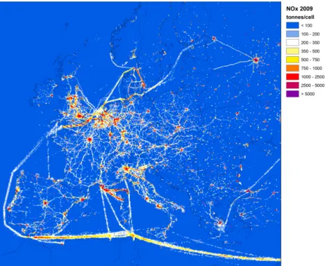
Figure 8.Spatially distributed NOxemissions from the year 2009 for all sources.
Poland and the Netherlands are shown (Fig. 7). In Poland, high EC emissions resulted from coal and wood combustion in the residential sector, which are much less relevant for the Netherlands. Total emissions from the road transport sector in the Netherlands and Poland are quite similar – the larger fleet size in Poland is more or less compensated by the lower share of diesel in the fuel mix.
3.3 Spatial distribution
The result of spatially distributing the emissions using the various proxies is shown for NOxand EC (< 2.5 µm) for the
year 2009 (Figs. 8 and 9, respectively). The major cities, ma-jor transport routes and shipping routes at sea can be identi-fied as important sources in these maps.
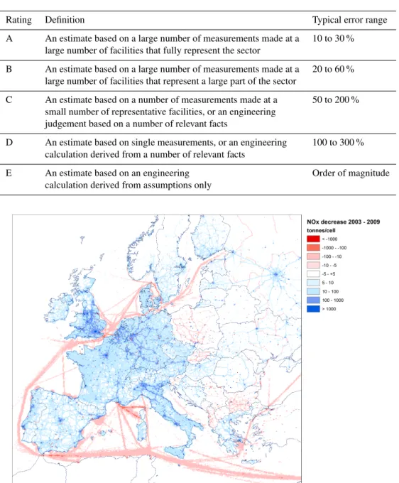
Figures 10 and 11 show also NOxand EC (< 2.5 µm), but
now the difference from 2003 to 2009. Positive numbers (blue colour in the maps) indicate a decrease in emissions
from 2003 to 2009, while negative numbers (red colour) show an increase in emissions. For NOx, it is shown that
most land-based emissions decrease, but in some countries in eastern Europe an increase is seen, e.g. in road transport for Poland, Slovak Republic and Bulgaria.
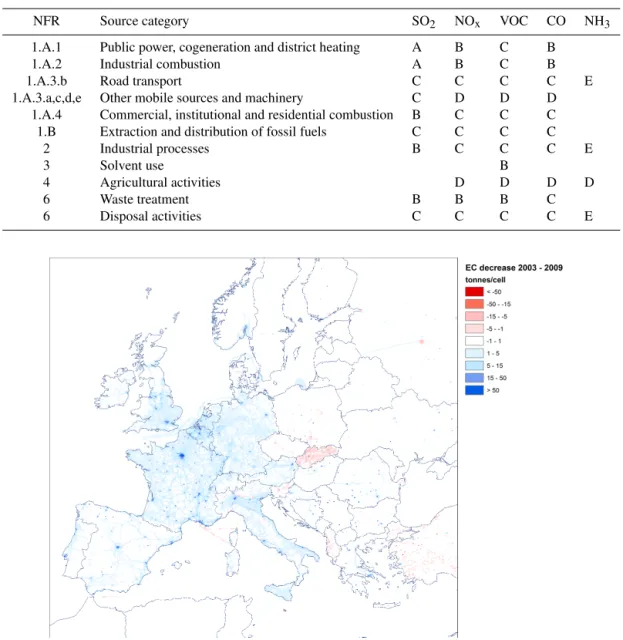
For fine particulate EC emissions are decreasing in most countries, but also increases are found especially in eastern Europe and at sea. Highest reductions are achieved in cities and urban areas, since the initial 2003 emissions in these re-gions were higher. Increases can be due to a growth in ac-tivity – e.g. for the Slovak Republic, the increase is due to higher reported emissions of PM2.5 from road transport in
2009 compared to 2003. Emissions from international ship-ping increased on all seas (CEIP, 2012).
Figure 9.Spatially distributed EC emissions (fine mode) from the year 2009 for all sources.
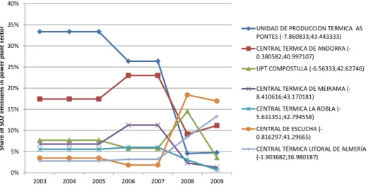
used on an annual basis for the distribution of the emissions over the various point sources. As an example, the share of each major power plant in the total SO2emission from the
power plant sector in Spain is shown in Fig. 12. The largest emitters in 2003 have reduced their emissions drastically. This causes some of the less important plants to become rel-atively more important, even though their absolute emission did not change. It was confirmed that in these specific cases for Spain, the power plants switched fuel (using coal with less or no sulfur) or installed advanced control technologies for desulfurization. The use of annual E-PRTR data for these large point sources enables us to reflect these changes from year to year. As mentioned earlier, for the years 2003, 2005 and 2006 no point source information was available and the closest year available has been used instead.
3.4 Uncertainties
A typical emission inventory is compiled by collecting ac-tivity data and appropriate emission factors, according to the EMEP/EEA Guidebook (EEA, 2013):
Emissionpollutant=
X
activitiesActivity rateactivity× (1)
Emission factoractivity,pollutant
Although for some sectors the equation to be used to es-timate emissions is more complicated than a simple mul-tiplication of a variable (Activity rateactivity) and a
parame-ter (Emission factoractivity,pollutant), in general such a simple
equation can be used to obtain uncertainty estimates. For a
more detailed treatment of the uncertainty calculations see EEA (2013, Chapter A5, Uncertainties).
For activity data like statistics the overall estimate of un-certainty would be 5–10 % (EEA, 2013). However, for the emission factors this is much more complicated as it may differ by source and pollutant and is often not known. To tackle this issue, a system has been developed that rates the uncertainty of emission factors (Table 4). This system makes it possible to give different ratings to various pollutant emis-sion factors for a single source. As an illustration and indi-cation of uncertainty we reproduce the general assessment of emission factors uncertainties for European emissions (Ta-ble 5). The values in Ta(Ta-ble 5 provide a good approximation of the uncertainty in the TNO_MACC-II emission inventory, as well as the country reported data being at the base of our inventory. A more elaborate uncertainty analysis has not been made. Although such an uncertainty analysis is desir-able it should be realized that it is a highly complicated and time consuming endeavour. The mixing of the different ap-proaches to obtain the most reliable and consistent data set asks for a complicated weighing of uncertainties, that differs country by country. Moreover, it may not be entirely feasible as we use country reported data (for good reasons) but the detailed information such as uncertainty in national statis-tics and often country-specific emission factors is simply not available.
The PM10, NOx, SO2 and NH3 emissions data
Table 4.Uncertainty rating definitions used for air pollutants in the Emission Inventory Guidebook (source: EEA, 2013).
Rating Definition Typical error range
A An estimate based on a large number of measurements made at a 10 to 30 % large number of facilities that fully represent the sector
B An estimate based on a large number of measurements made at a 20 to 60 % large number of facilities that represent a large part of the sector
C An estimate based on a number of measurements made at a 50 to 200 % small number of representative facilities, or an engineering
judgement based on a number of relevant facts
D An estimate based on single measurements, or an engineering 100 to 300 % calculation derived from a number of relevant facts
E An estimate based on an engineering Order of magnitude
calculation derived from assumptions only
Figure 10.Change in NOxemissions between 2003 and 2009 in Europe, for all sources.
Environment Agency (EEA, 2011) assesses the uncertainty in emissions for the SO2, NOxand NH3as follows:
– Sulfur dioxide emission estimates in Europe are thought to have an uncertainty of about 10 % as the sulfur emit-ted comes from the fuel burnt and therefore can be more accurately estimated. However, because of the need for interpolation to account for missing data the complete data set used here will have higher uncertainty. EMEP has compared modelled (using emission inven-tory data) and measured concentrations throughout Eu-rope (EMEP, 1998). From these studies differences in the annual averages have been estimated in the order of 30 % consistent with an inventory uncertainty of 10 %
(there are also uncertainties in the measurements and especially the modelling).
– Nitrogen oxide emission estimates in Europe are thought to have an uncertainty of about±20 % (EMEP,
2009), as the NOx emitted comes both from the fuel
burnt and the combustion air and so cannot be estimated accurately from fuel nitrogen alone. However, because of the need for interpolation to account for missing data, the complete data set used will have higher uncertainty. – Ammonia emissions are relatively uncertain. NH3
Table 5.Main relevant NFR source categories with applicable quality data ratings (source: EEA, 2013).
NFR Source category SO2 NOx VOC CO NH3
1.A.1 Public power, cogeneration and district heating A B C B
1.A.2 Industrial combustion A B C B
1.A.3.b Road transport C C C C E
1.A.3.a,c,d,e Other mobile sources and machinery C D D D
1.A.4 Commercial, institutional and residential combustion B C C C
1.B Extraction and distribution of fossil fuels C C C C
2 Industrial processes B C C C E
3 Solvent use B
4 Agricultural activities D D D D
6 Waste treatment B B B C
6 Disposal activities C C C C E
Figure 11.Change in EC (< 2.5 µm) emissions between 2003 and 2009 in Europe, for all sources.
agricultural sources – which account for the vast major-ity of NH3emissions. It is estimated that they are around ±30 % (EMEP, 2011). The trend is likely to be more ac-curate than the individual absolute annual values – the annual values are not independent of each other.
The above estimates are in line with De Leeuw (2002) (but also largely based on the same methodologies) who reported uncertainties in emissions as about 50 % for NH3, VOC and
CH4. NOx emission estimates in Europe were thought to
have an uncertainty of about±30 % and SO2emission
esti-mates in Europe were thought to have an uncertainty of about
±10 % as the sulfur emitted comes from the fuel burnt and
so can be relatively accurately estimated. However, because of the need for interpolation to account for missing data the
complete EU data set studied by De Leeuw (2002) will have higher uncertainty.
More recently, Nielsen et al. (2014) reported Danish un-certainty estimates for the total emissions of air pollutants from Denmark. The Danish uncertainty estimates were still based on the simple Tier 1 approach described by Pulles and Van Aardenne (2004). The uncertainty estimates are based on uncertainties for fuel consumption and emission factors for each of the main SNAP source categories. Un-certainty in total Danish emissions for pollutants as used in the TNO-MACC_II inventory were estimated as SO2(16 %),
NOx(39 %), NMVOC (23 %),CO (42 %), NH3(29 %), PM10
(289 %) and PM2.5(347 %) (Nielsen et al., 2014). For SO2,
NOx and NH3 this is all rather consistent but it should be
0% 5% 10% 15% 20% 25% 30% 35% 40%
2003 2004 2005 2006 2007 2008 2009
S
h
are
o
f S
O
2
emi
ss
io
n
s
in
p
o
we
r
p
lan
t
sect
o
r UNIDAD DE PRODUCCION TERMICA AS PONTES (-7.860833;43.443333)
CENTRAL TERMICA DE ANDORRA (-0.380582;40.997107)
UPT COMPOSTILLA (-6.56333;42.62746)
CENTRAL TERMICA DE MEIRAMA (-8.410616;43.170181)
CENTRAL TERMICA LA ROBLA (-5.631351;42.794558)
CENTRAL DE ESCUCHA (-0.816297;41.29665)
CENTRAL TÉRMICA LITORAL DE ALMERÍA (-1.903682;36.980187)
Figure 12.Contribution of the top-7 SO2emitting power plants in Spain in 2003 to the annual total SO2emissions from the power plant sector.
because the data to do a complete detailed uncertainty anal-ysis of all relevant source are simply not available. Remark-able in the reporting by Nielsen et al. (2014) is the high un-certainty in PM emissions. This is mostly due to the high uncertainty in emission factors for residential combustion which is one of the key sources of PM in Europe. However, it is not so much uncertainty as well as definition of PM mea-surement methodology which is especially variable for resi-dential combustion stoves (Nussbaumer et al., 2008). Since different countries use different methodologies this results in extremely high uncertainty of the order of 200–300 % as re-ported by Nielsen et al. (2014).
Independent of the uncertainty in national total emissions is the uncertainty in spatial distribution of the emissions within a country which is done using proxy data. Some prox-ies are more accurate than others. For example a point source database for power plants is fairly accurate although some uncertainty is present related to the specific fuel use, fuel quality and operation times. For some other proxies, e.g. the population density used to distribute the emission from wood stoves, the accuracy of this proxy is not known as we do not really know where the wood stoves are. The uncertainty of using such a proxy increases when going from a large to a smaller grid size. Moreover, for some countries the proxy data like road networks or industrial activity may more de-tailed than for other countries. Hence the uncertainty may vary from country to country.
4 Conclusions
A model-ready emission inventory at high spatial resolution for UNECE-Europe for 7 consecutive years (2003–2009) was constructed, which combines the advantage of using of-ficial reported emissions to the extent possible. For air qual-ity modelling and environmental impact assessment studies,
a good understanding of the magnitude and location of the sources of pollution is of crucial importance for deriving pol-icy conclusions. The main advantages of this inventory are:
– We use source sector-specific data in a harmonized way, which allows both tracking of sources in the modelled data as well as trend analysis without artifacts such as differences between annual reporting years. For in-stance, NMVOC and NOx from agriculture were
ex-cluded for all countries as reporting was found to be very inconsistent.
– The application of a consistent gridding methodology for all countries ensures patterns across borders do not show sudden changes or jumps – e.g. consistent land use and animal density maps to distribute agricultural emissions.
– To model particulate matter concentration and fate, models need to break down PM into components with different behaviour. We now provide such data which are not available from the official reporting.
– By using the point source data from E-PRTR and EPER, better locations of point sources were brought into the database. Moreover, the point source gridding data is now year-specific, whereas earlier the 2005 distribution was used as a proxy for all years.
– Emissions in ports were added in a harmonized way for the whole of Europe.
– Finally, since the data are as much as possible (given our quality criteria) from the official reported data, the data can be readily used for policy evaluation.
Our emission data set has been compared to other emis-sion inventories to assess the quality of the inventory. Since GAINS was a primary data source used, a good match was found with this inventory. Between our inventory and EDGAR differences were found, which can partly be ex-plained by allocation issues and by a somewhat different do-main definition.
Uncertainties in emission inventories are difficult to quan-tify, especially when multiple sources are combined. General approaches to uncertainty exist, but data collection is difficult especially at European scale.
A potentially new way to address uncertainty in large point sources is by comparing the emission maps with satellite measurement. A first comparison between OMI satellite data and SO2source strength of major point sources (Visschedijk
et al., 2012) revealed that for some major point sources in eastern Europe, no OMI signal was found, which could indi-cate that the point source closed, or changed fuel. The result-ing information from this type of comparisons is very useful to further improve the point source databases in the future.
All in all, this paper presents a significantly improved spa-tially explicit emission data set for the European domain. However, one should bear in mind the limitations of the Eu-ropean scale emission inventory. Since the spatial distribu-tion of nadistribu-tional emissions is done using a generic system of point sources and proxies, differences with other inventories may exist, especially when zooming in to the local scale such as a large city or urban area.
A next step would be to include the “semi-natural” sources in our emission inventory, which are not covered by official inventory data (e.g. resuspension of dust and NOxemissions
from soils). With decreasing emissions from most anthro-pogenic sources, these become increasingly important for the comparison between modelled and observed concentrations.
The Supplement related to this article is available online at doi:10.5194/acp-14-10963-2014-supplement.
Acknowledgements. This research has been funded by the FP7 projects MACC and MACC-II. The authors thank the Centre for Emission Inventories and Projections (CEIP) and the European Environment Agency (EEA) for making reported data available in a comprehensive format. The IIASA GAINS and JRC EDGAR teams are gratefully acknowledged for important emission inventory work which was used in the present study.
Edited by: S. Galmarini
References
Amann, M.: Integrated assessment tools: The Greenhouse and Air Pollution Interactions and Synergies (GAINS) model, in: Atmo-spheric Pollution and Climate Change: How to address both chal-lenges effectively together?, 73–76, 2009.
Amann, M., Bertok, I., Borken-Kleefeld, J., Cofala, J., Heyes, C., Hoeglund-Isaksson, L., Klimont, Z., Nguyen, B., Posch, M., Rafaj, P., Sandler, R., Schoepp, W., Wagner, F., and Winiwater, W.: Cost-effective control of air quality and greenhouse gases in Europe: Modelling and policy applications, Environ. Modell. Softw., 12, 1489–1501, 2011.
Centre for Emission Inventories and Projections: Reported emissions by Parties under the Convention for Long-Range Transboundary Air Pollution, http://www.ceip.at/ webdab-emission-database/officially-reported-emission-data/, date of download 12 March 2012, 2012.
Cotteleer, A. and Van der Tak, C.: MARIN’s emission inventory for North Sea shipping 2009: Validation against ENTEC’s in-ventory and extension with port emissions, 2nd final report No. 25300-1-MSCN Rev. 2, Maritime Research Institute Netherlands MARIN, Wageningen, the Netherlands, 2009.
De Ceuster, G., Franckx, L., van Herbruggen, B., Logghe, S., van Zeebroeck, B., Tastenhoye, S., Proost, S., Knockaert, J., Williams, I., Deane, G., Martino, A., and Firello, D.: TREMOVE 2.30 Model and Baseline description, Final Report, Transport and Mobility Leuven, http://www.tremove.org (last access: 16 February 2009), 2005.
Denier van der Gon, H. A. C., Visschedijk, A., Van der Brugh, H., and Dröge, R.: A high resolution European emission database for the year 2005, a contribution to the UBA-project PAREST: Particle Reduction Strategies, TNO report TNO-034-UT-2010-01895_RPT-ML, Utrecht, 2010.
EMEP: Transboundary Acidifying Air Pollution in Europe, Part 1: Estimated dispersion of acidifying and eutrophying compounds and comparison with observations, EMEP/MSC-W Report 1/98, July 1998.
EMEP: Transboundary Acidification, Eutrophication and Ground Level Ozone in Europe in 2009, EMEP Status Report 2011, EMEP Report 1/2011, 2011.
European Commission: Council Directive 96/61/EC of 24 Septem-ber 1996 concerning integrated pollution prevention and control, Official Journal L 257, 26–40, European Commission, 1996. European Commission: Directive 2012/33/EU of the European
Par-liament and of the Council of 21 November 2012 amending Council Directive 1999/32/EC as regards the sulfur content of marine fuels, Official Journal L 327, 1–13, European Commis-sion, 2011.
European Environment Agency: The European environment – state and outlook 2010: synthesis, European Environment Agency, Copenhagen, 2010.
European Environment Agency: Emissions of primary particles and secondary particulate matter precursors, Indicator code CSI 003, Published 11 November 2008, Last modified: 7 July 2011, 02:39 p.m., http://www.eea.europa.eu/data-and-maps/indicators/ ds_resolveuid/781d346e34436a4aacf75c63e7288078, 2011. European Environment Agency: Evaluation of progress under the
European Environment Agency: Reported emissions by Parties un-der the Convention for Long-Range Transboundary Air Pollution and the UN Framework Convention on Climate Change, date of download 3 March 2012, 2012b.
European Environment Agency: EMEP/EEA Air Pollutant Emis-sion Inventory Guidebook, 2013 edition, http://www.eea. europa.eu/publications/emep-eea-guidebook-2013 (last access: 9 September 2013), 2013.
Intergovernmental Panel on Climate Change: IPCC Guidelines for National Greenhouse Gas Inventories, Intergovernmental Panel on Climate Change, Japan, 2006.
International Institute for Applied Systems Analysis: GAINS de-tailed emissions by source and activity, http://gains.iiasa.ac.at/ gains/EUN/index.login?logout, PRIMES baseline scenario 2009, download date 19 June 2012, 2012.
Joint Research Centre: TRANSTOOLS, Tools for transport fore-casting and scenario testing, Version 1, http://energy.jrc.ec. europa.eu/transtools/index.html (last access: 1 December 2008), 2005.
Joint Research Centre: Emission Database for Global Atmospheric Research (EDGAR) v4.2, http://edgar.jrc.ec.europa.eu (last ac-cess 24 May 2012), 2011.
Kuenen, J. J. P., Denier van der Gon, H. A. C., Visschedijk, A., Van der Brugh, H., and Van Gijlswijk, R.: MACC European emission inventory for the years 2003–2007, TNO report TNO-060-UT-2011-00588, Utrecht, 2011.
Leeuw, F. de: A set of emission indicators for long-range trans-boundary air pollution, Environmental Science and Policy, 5, 135–145, 2002.
Nielsen, O.-K., Winther, M., Mikkelsen, M. H., Hoffmann, L., Nielsen, M., Gyldenkærne, S., Fauser, P., Plejdrup, M. S., Al-brektsen, R., Hjelgaard, K., and Bruun, H. G.: Annual Danish Informative Inventory Report to UNECE, Emission inventories from the base year of the protocols to year 2012, Aarhus Univer-sity, DCE – Danish Centre for Environment and Energy, 759 pp. Scientific Report from DCE – Danish Centre for Environment and Energy No. 94, http://dce2.au.dk/pub/SR94.pdf, 2014. Ntziachristos, L., Gkatzoflias, D., Kouridis, C., and Samaras, Z.:
COPERT: A European road transport emission inventory model, in: Information Technologies in Environmental Engineering, En-vironmental Science and Engineering, edited by: Athanasiadis, I. N., Mitkas, P. A., Rizzoli, A. E., and Marx Gómez, J., Springer-Verlag, Heidelberg, 491–504, doi:10.1007/978-3-540-88351-7_37, 2009.
Nussbaumer, T., Klippel, N., and Johansson, L.: Survey on measure-ments and emission factors on particulate matter from biomass combustion in IEA countries, 16th European Biomass Confer-ence and Exhibition, 2–6 June 2008, Valencia, Spain – Oral Pre-sentation OA 9.2, 2008.
Olivier, J. G. J., Bouwman, A. F., Berdowski, J. J. M., Veldt, C., Bloos, J. P. J., Visschedijk, A. J. H., Van der Maas, C. W. M., and Zandveld, P. Y. J.: Sectoral emission inventories of greenhouse gases for 1990 on a per country basis as well as on 1◦ ×1◦, Environmental Science and Policy 2, 241–263, 1999.
Pouliot, G., Pierce, T., Denier van der Gon, H., Schaap, M., Moran, M., and Nopmongcol, U.: Comparing emission inventories and model-ready emission databases between Europe and North America for the AQMEII project, Atmos. Environ., 53, 4–14, 2012.
Pulles, T. and Aardenne, J. V.: Good Practice Guidance for LRTAP Emission Inventories, http://www.eea.europa.eu/publications/ EMEPCORINAIR4/BGPG.pdf, 2004.
Schaap, M., Sauter, F., Timmermans, R. M. A., Roemer, M., Velders, G., Beck, J., and Builtjes, P. J. H., The LOTOS-EUROS model: description, validation and latest developments, Int. J. En-viron. Pollut., 32, 270–290, 2008.
Schöpp, W., Amann, M., Cofala, J., Heyes, C., and Klimont, Z.: Integrated assessment of European air pollution emission control strategies, Environ. Modell. Softw., 14, 1–9, doi:10.1016/S1364-8152(98)00034-6, 1999.
Timmermans, R. M. A., Denier van der Gon, H. A. C., Kuenen, J. J. P., Segers, A. J., Honoré, C., Perrussel, O., Builtjes, P. J. H., and Schaap, M.: Quantification of the urban air pollution increment and its dependency on the use of down-scaled and bottom-up city emission inventories, Urban Climate, 6, 44–62, 2013.
UNECE: Guidelines for Estimating and Reporting Emission Data under the Convention on Long-range Transboundary Air Pol-lution, ECE/EB.AIR/80, Air Pollution studies No. 15, United Nations, New York and Geneva, http://www.unece.org/env/ documents/2003/eb/air/ece.eb.air.80.E.pdf, 2003.
Van Loon, M., Tarrason, L., and Posch, M.: Modelling base cations in Europe, MSC-W Technical Report 2/2005, available at: http://emep.int/publ/reports/2005/emep_technical_ 2_2005.pdf (last access: 1 December 2008), 2005.
Visschedijk, A. J. H., Zandveld, P. Y. J., and Denier van der Gon, H. A. C.: A high resolution gridded European emission database for the EU Integrate Project GEMS, TNO report 2007-A-R0233/B, TNO, Utrecht, the Netherlands, 2007.
Visschedijk, A. J. H., Denier van der Gon, and H. A. C., and Dröge, R.: A European high resolution and size-differentiated emission inventory for elemental and organic carbon for the year 2005, TNO-034-UT-2009-00688_RPT-ML, TNO, Utrecht, the Nether-lands, 2010.