Rev. IBRACON Estrut. Mater. vol.4 número4

(1)

This work presents a numerical model for 3D analyses through the inite element method of reinforced concrete structures subjected to monotonic loads. The proposed model for concrete is orthotropic and uses the equivalent uniaxial strain concept. The equivalent uniaxial stress-strain relation is generalized to take into account the triaxial stress conditions. The parameters used in the equivalent uniaxial stress-strain curve are determined from the failure surface deined in the principal stress space. The implementation in inite elements is based on the consideration of smeared cracks with cracks rotating according to the directions of the principal stresses. Also, an embedded reinforcement model was implemented to represent existent reinforcing bars. Finally, some results are compared with experimental data from the literature to demonstrate the validity of the numerical model developed.

Keywords: reinforced concrete; inite element method; constitutive models; orthotropic model.

Este trabalho apresenta um modelo numérico para análise tridimensional de estruturas de concreto armado submetidas a cargas monótonas. O modelo proposto para o concreto é um modelo ortotrópico e utiliza o conceito de deformação uniaxial equivalente. A relação tensão-deformação uniaxial equivalente é generalizada para levar em consideração as condições triaxiais de tensão. Os parâmetros usados na curva tensão-defor-mação uniaxial equivalente são determinados a partir da superfície de ruptura deinida no espaço de tensões principais. Também, implementou-se um modelo de armadura incorporada para repreimplementou-sentar as barras de armadura. Por im, apreimplementou-sentam-implementou-se resultados comparativos com ensaios experimentais e analíticos para demonstrar a validade do modelo numérico.

Palavras-chave: concreto armado; método dos elementos initos; modelos constitutivos; modelo ortotrópico.

A 3D inite element model for reinforced concrete

structures analysis

Modelo 3D de elementos initos para análise

de estruturas de concreto armado

G. F. F. BONO a

giuliana.franca@gmail.com

A. CAMPOS FILHO b

americo@ufrgs.br

A. R. PACHECO b

apacheco@ufrgs.br

a_{Graduate Program in Civil and Environmental Engineering, Federal University of Pernambuco, giuliana.franca@gmail.com, BR 104, Km 59, S/N,}

Nova Caruaru, 55002-970, Caruaru, Pernambuco, Brazil

b_{Graduate Program in Civil Engineering, Federal University of Rio Grande do Sul, americo@ufrgs.br, apacheco@ufrgs.br, Av. Osvaldo Aranha - 99,}

3º andar, 90035-190, Porto Alegre, Rio Grande do Sul, Brazil

Received: 07 Feb 2011 • Accepted: 03 Jun 2011 • Available Online: 07 Oct 2011

Abstract

(2)

1. Introduction

The implementation of inite element models to investigate rein -forced concrete structures has been the subject of many studies in the last years (Patrick and Sharon Huo [1], Kim and Aboutaha [2], Park and Aboutaha [3], Hoque et al. [4], Smadi and Belakh -dar [5], Souza et al. [6], Shayanfar and Saiey [7], Manzoli et al. [8]). In several of these studies, a fundamental matter has been how to precisely deine concrete’s behavior when a multiaxial state of stress is in place. This task has been dificult because of the behavioral complexity of the material due to a series of factors, among which, these can be pointed out: concrete presents a non-linear stress-strain relation; cracks tend to form when concrete is subjected to tensile stresses; concrete is subjected to creep and shrinkage; concrete’s behavior is dependent of its load history; and concrete presents a volumetric expansion when near collapse. In the last decades, numerous constitutive models were developed for the analysis of concrete structures. However, most of them, in general, can describe only certain aspects of concrete’s behavior, severely limiting their application. Among the most important char-acteristics a model for concrete must present, the following can be highlighted: to allow a general and precise representation of its real mechanical behavior; to employ a formulation that is clear to understand; and to make viable the implementation of a robust algorithm, stable enough for a nonlinear behavior determination. In this context, the objective of this work is to present a computa -tional model to analyze the behavior of reinforced concrete ele -ments subjected to multiaxial stress states. The constitutive mod-els adopted for concrete and steel are herein described in details, and have been implemented in a computational code, developed by Bono [9], to analyze reinforced concrete structures through the Finite Element Method. Linear and quadratic isoparametric hexa-hedral elements can be chosen to model reinforced concrete struc -tures, with the embedded reinforcing model proposed by Elwi and Hrudey [10] extended to the 3D case being used to represent the existent reinforcing bars.

2. Constitutive model for the concrete

In this work, an orthotropic nonlinear elastic constitutive model is used to represent the concrete’s behavior. Among the models that have been already developed in this category, there is the one presented by Darwin and Pecknold [11] for plane stress state analyses. Elwi and Murray [12] continued the development of this model, extending its applicability to the 3D case. Afterwards, the model was further developed by Balan et al. [13], Balan et al. [14], Kwon [15], and Kwon and Spacone [16].

The orthotropic model proposed is based on the work by Kwon [15], being capable of simulating the response of concrete under a multiaxial stress state. Nevertheless, some modiications have been implemented in the original model in order to further improve it, which are appropriately commented later along with the model’s formulation.

2.1 Tridimensional constitutive law

Originally, Darwin and Pecknold [11] developed a numerical pro -cedure to analyze the response of concrete under biaxial stress

states by considering the orthotropic axes parallel to the directions of the updated principal stresses. Elwi and Murray [12] extended that model to tridimensional analyses. The stress-strain relation can be expressed by:

(1)

=

_o

σ D ε

where the stress vector, s, and the strain vector, e, can be given by:

(2)

1 2 3 12 23 31

s

t

ì

ü

ï

= í ý

ï

î

þ

σ

and

1 2 3 12 23 31

e

g

ì

ü

ï

= í ý

ï

î

þ

ε

The constitutive matrix for an orthotropic material, D_o, can be

de-termined by:

(3)

(

) (

)

(

) (

)

(

) (

)

1

0

1

0

1

0

1

0

1 23 32 1 21 23 31 1 31 21 32 2 12 13 32 2 13 31 2 32 12 31 3 13 12 23 3 23 13 21 3 12 21

c 12 c

23 c 31 c

E

G

n n

n n n

n n

n n n

n n

W

é

-

+

ù

ê

₊

_-

₊

ú

ê

ú

ê

+

-

ú

= ê

ú

W

ê

ú

ê

_W

ú

ê

ú

W

ê

ú

ë

û

o

D

where

Ωc = 1 – ν21ν12 – ν31ν13 – ν32ν23 – ν12ν23ν31 – ν21ν32ν13;

E_i – is the secant modulus of elasticity in the orthotropic direction i (i = 1, 2, 3);

νij – is the Poisson’s ratio (i, j = 1, 2, 3);

G_ij – is the shear modulus of elasticity on the i-j plane (i, j = 1, 2, 3). The shear moduli, G_ij, can be expressed by:

(4)

(

1 ) (

1 )

i j ij

i ij j ji

E E

G

E

n

E

n

=

+

If the orthotropic axes are considered parallel to the directions of the updated principal stresses, then the constitutive relation can be reduced to:

(5)

(

) (

)

(

) (

)

(

) (

)

1

1 ₁

1

1 1 23 32 1 21 23 31 1 31 21 32 1 2 2 12 13 32 2 13 31 2 32 12 31 2

c

3 3 13 12 23 3 23 13 21 3 12 21 3

E

s

n n

n n n

e

s

n n n

n n

n n n

e

s

n n n

n n

e

-

+

é

ù

ì ü

ï ï

₌

ê

₊

_-

₊

ú

ï ï

í ý

_W

_ê

_ú

í ý

ï ï

_ê

₊

_-

_ú

ï ï

(3)

The equivalent uniaxial strains are used for determination of con-crete’s properties, i.e., the secant moduli of elasticity and the Pois -son’s ratios, which are used in Equation (5). Nevertheless, it can be noticed from Equation (6) that, to obtain the equivalent uniaxial strains for a nonlinear material, the secant moduli of elasticity, E_i, are needed in the directions of the three principal stresses, be -ing necessary the use of an iterative process for determination of these variables (see section 2.8).

2.3 Equivalent uniaxial stress-strain curves

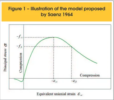
As mentioned before, the adopted model for concrete follows the work of Darwin and Pecknold [11], admitting that the 3D con-stitutive law can be separated in three uniaxial relations, with actual stresses being functions of equivalent uniaxial strains. Elwi and Murray [12] used an expression by Saenz [17] to de -scribe equivalent uniaxial stress-strain relations, which was both adopted for concrete’s compressive and tensile response (see Figure 1):

(9)

2 3

1

ui i

ci

i ci

ui ui ui

i i i

ci ci ci

K

f

A

B

C

e

s

e

æ

ö

ç

÷

è

ø

=

æ

ö

æ

ö

æ

ö

+

_ç

_÷

+

_ç

_÷

+

_ç

_÷

è

ø

è

ø

è

ø

where In relation (5), the values of the secant moduli of elasticity, E_i,

and the Poisson’s ratios, νij, have to be determined. These

val-ues are obtained from the uniaxial stress-strain curves for the concrete using the concept of equivalent uniaxial strain, which is detailed next.

2.2 Equivalent uniaxial strain

In a multiaxial stress state, the actual strain in a given direction is not only function of the stress in that direction, but also of the stresses acting in the other orthogonal directions. This makes the determination of the 3D response of concrete a complex task to perform. In order to make it an easier task, the concept of equiva -lent uniaxial strain can be used, a concept originally introduced by Darwin and Pecknold [11] for 2D analyses.

Darwin and Pecknold [11] considered this procedure to be an in -genious scheme to separate the 2D response of concrete in two uniaxial curves, making it easier to determine the material’s behav-ior. The technique provided an alternative to separate the effects of the Poisson’s ratios of each strain, allowing a good approxima-tion of experimental data. The equivalent uniaxial strains can be determined by:

(6)

i ui

i

E

s

e =

where

σi – is the current principal stress in the orthotropic direction i;

E_i – is the secant modulus of elasticity in the orthotropic direction i, with i = 1, 2, 3 for 3D analyses.

Kwon [15] also used the concept of equivalent uniaxial strain for 3D analyses in concrete, rewritting relation (5) in the following form:

(7)

0

1 1 u1

2 2 u2

3 3 u3

E

s

e

s

e

s

e

ì ü é

ù ì ü

ï ï

₌

ê

ú

ï ï

í ý

_ê

_ú

í ý

ï ï

_ê

_ú

ï ï

î þ ë

û î þ

and the equivalent uniaxial strains are then given by:

(8)

(

) (

)

(

) (

)

(

) (

)

1 1

1 ₁

u1 23 32 1 21 23 31 2 31 21 32 3 c

u2 12 13 32 1 13 31 2 32 12 31 3 c

u3 13 12 23 1 23 13 21 2 12 21 3 c

e

n n e n n n e n n n e

W

e

n n n e

n n e n n n e

W

e

n n n e n n n e

n n e

W

=

é

_ë

-

+

ù

_û

=

é

_ë

+

+ -

+

ù

_û

=

é

_ë

+

+ -

ù

_û

The principal stresses σ₁, σ₂, and σ₃ can be obtained from the uniax -ial constitutive relations [Equation (6)], using the equivalent uniax-ial strains ε_u1, ε_u2, and ε_u3. Therefore, the introduction of these equiva-lent uniaxial strains allows a representation of the triaxial behavior of the concrete through three independent stress-strain curves. It is worth mentioning that these equivalent uniaxial strains are not actual strains, but ictitious strains deined in the updated directions of the principal stresses, being accumulated in these directions. Thus, ε_ui does not give a strain history in a ixed di -rection, but rather in an always changing direction with the up -dated state of principal stresses (Darwin and Pecknold [11]).

(4)

(

)

(

)

2

1

i

i i

K

C K

K

s

e e

-=

--

; Di = 0.

The other variables were deined in Equations (9)-(10).

The use of the Popovics-Saenz curve (Equation (11)) as an equiv-alent uniaxial relation gives excellent results for plain concrete. Nevertheless, for reinforced concrete elements it has not shown to be adequate to take into account the collaboration of concrete between cracks (tension-stiffening). Therefore, for the proposed model herein, the Popovics-Saenz curve is used to describe only the response in compression of concrete under monotonic loads, as illustrated in Figure 2, and, for the response in tension, the for -mulation described next is used. When εui ≤εci:

(12)

s

i

= E

o

e

ui

with i = 1, 2, 3.

E_o – is the initial modulus of elasticity;

εui – is the equivalent uniaxial strain in the orthotropic direction i;

f_ci – is the concrete strength or the peak stress;

εci – is the strain that corresponds to fci, i.e., it is the peak strain.

f_i, ε_i – are the stresses and strains at the control point in the curve’s descending branch.

The proposed curve by Saenz [17] has been considerably used as a stress-strain relation for concrete, with only one expres-sion representing both ascending and descending branches. However, this curve works well only when E_o/E_ci ³ 2 (where E_ci = f_ci/ε_ci), i.e., when the secant modulus of elasticity at the peak point, E_ci, is not larger than half of the initial modulus of elastic-ity, E_o. When this condition is not satisfied, the curve will pres -ent two curvatures between the origin and the peak point. This problem can be partially corrected by fixing E_o/E_ci to a value of 2, independently of the actual relation between the two moduli (Balan et al. [14]).

Popovics [18] proposed another curve to deine concrete’s stress-strain relation, which is expressed by:

(10)

(

)

1

i

ui i

ci

i ci R

ui i

ci

K

f

K

e

s

e

æ

ö

ç

÷

è

ø

=

æ

ö

+

_{- ç ÷}

è

ø

_with

_i

_{= 1, 2, 3.}

where R_i = K_i / (K_i – 1) and the other variables have already been deined in Equation (9). This curve approximates well the actual initial stiffness of concrete in the ascending branch. However, it does not adjust well to experimental data when descending. To avoid any limitation in the deinition of the equivalent uniaxial curve, Kwon [15] proposed a modiication in the curve used by Elwi and Murray [12]: two curves are used to describe the responses in tension and in compression of concrete. The curve proposed by Popovics [18] should describe the ascending branch until the peak point, while the curve proposed by Saenz [17] should be used in the response of the descending branch. The combination of the models by Popovics [18] and Saenz [17], named as Popovics-Saenz curve, from Equations (9) to (10), can then be expressed by the following relation:

(11)

2 3

1

i

ui i

ci

i ci R

ui ui ui ui

i i i i

ci ci ci ci

K

f

A

B

C

D

e

s

e

æ ö

ç ÷

è ø

=

æ ö æ ö

æ ö

+

_{ç ÷ ç ÷}

+

_{ç ÷}

+

_{ç ÷}

è ø è ø

è ø

_with

_{i=1, 2, 3.}

– Ascending: If ui

1

ci

e

æ

ö

£

ç

÷

è

ø

: Ai = Bi = Ci = 0; Di = Ki – 1;

– Descending: If ui

1

ci

e

æ

ö

>

ç

÷

è

ø

: Ai = Ci+Ki–2; Bi = 1 – 2Ci;

Figure 2 – Stress-strain curves for concrete

subjected to monotonic

(5)

But when εui > εci, the valid expression is:

(13)

(1

)

0.01

ui

i t ci

f

e

s

=

a

with

i

= 1, 2, 3.

where

αt – is a coefficient for reduction of cracking stresses, and the

other variables were defined in Equation(9).

The variable εctu, introduced in Figure 2, indicates the limiting strain

for which the collaboration of concrete between cracks should not be considered any longer. In this study, in order to allow a bet-ter agreement with experimental data, a value of 0.01 has been adopted for the strain ε_ctu, as indicated in Equation (13), while the value of parameter α_t depended on the element analyzed.

In Equations (11) to (13), the expression proposed in CEB-FIP Model Code 1990 [19] was adopted for the initial modulus of elasticity, E_o. Through those three equations, the secant moduli of elasticity, used in Equation (6), could be deined by considering E_i = σ_i /ε_ui, with i = 1, 2, 3.

2.4 Failure surface of concrete

The determination of the variables K_i, K_εi, K_σi, used in Equation (11), which are functions of the peak stresses and strains, f_ci and ε_ci, is necessary for deinition of the three equivalent uniaxial curves. This peak stresses and strains, for a determined current stress state, are calculated from failure surfaces in the space of principal stresses (σ1, σ2, σ3).

Numerous formulations have been proposed as failure surfaces for concrete. A series of failure criteria was presented by Chen and Han [20] and by Menétrey and Willam [21], classifying these criteria according to the number of parameters that appear in the respective expressions.

Among the more used failure surfaces for description of

con-crete’s triaxial strength, there are the four-parameter surface by Ottosen [22] and the ive-parameter surface by Willam and Warnke [23]. These surfaces have been highly used because the failure points they determine are quite close to available ex-perimental data, as can be seen in Chen and Han [20]. There -fore, for the present model, the failure surfaces by Ottosen [22] and Willam and Warnke [23] were implemented for concrete. The equations used for these two surfaces are presented in details in the next sections.

2.4.1 The failure surface by Willam and Warnke

This failure surface can be expressed by the following equation:

(14)

f

(

s

_m

,

r

,

q

) =

r

–

r

_f

(

s

_m

,

q

) = 0

|

q

|

£

60

o

where

3

_oct

r

=

τ

– is the stress component perpendicular to the hydro -static axis;

ρf(σm, q) – deines the failure curve on deviatoric planes, being

determined by:

(15)

(

,

)

f m

s t

_v

r

s q

=

+

where

(

)

(

2 2

)

,

2 cos

m c c t

s

=

s

σ q

=

r r

−

r

q

(

)

(

)

1/ 2

,

2

m c t c

t

=

t

σ q

=

r

r r

−

u

(

)

(

2 2

)

2

(

)

2

,

4 cos

2

m c t c t

v

=

v

σ q

=

r

−

r

q

+

r

−

r

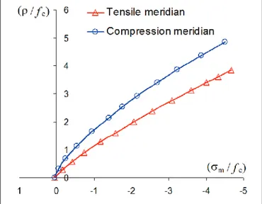
The ive-parameter surface by Willam and Warnke [23] presents parabolic curves for tensile and compression meridians (Figure 3) expressed by:

(16)

2

m

a a

0 1 t

a

2 t

s

= +

r

+

r

_{tensile meridian (}

_{q =}

₀

o

)

2 m

b b

0 1 c

b

2 c

s

= +

r

+

r

_{compression meridian (}

_{q =}

₆₀

o

)

where

σm – is the mean normal stress;

ρt, ρc – are stress components perpendicular to the hydrostatic axis

for q = 0o_and_q = 60o_{, respectively;}

a_o, a₁, a₂, b_o, b₁, b₂ – are material constants.

(6)

From Equation (16), the stress components perpendicular to the hydrostatic axis, ρ_c and ρ_t, are determined by:

(17)

(

)

1 ₄

2

t 1 1 2 0 m

2

a a a a

a

r

= -

é

_ë

+

-

s

ù

_û

for the tensile meridian.

(

)

1 ₄

2

c 1 1 2 0 m

2

b b b b

b

r

= -

é

_ë

+

-

s

ù

_û

for the compression meridian.

Since the two meridians should cross the hydrostatic axis at the same point, results that a₀ = b₀. Based on biaxial tests by Kupfer et al. [24] and other triaxial tests, the five parameters of the failure surface by Willam and Warnke [23] can be deter -mined from the following values on the failure surface (Chen and Han [20]):

f_c – uniaxial compression strength (q = 60o);

f_t = 0.1 f_c – uniaxial tensile strength (q = 0o);

f_cc = 1.15 f_c – biaxial compression strength (q = 0o);

(σmc, ρc) = (–1.95fc; 2.770fc) – conined biaxial compression strength

with σ₁ > σ₂ = σ₃;

(σmt, ρt) = (–3.90fc; 3.461fc) – conined biaxial compression strength

with σ₁ = σ₂ > σ₃.

From these failure states, the values of the five parameters used in the compression and tensile meridians, ρ_c and ρ_t, respectively, of the surface by Willam and Warnke [23] can be found: a₀ = b₀ = 0.1025; a₁ = –0.8403; a₂ = –0.0910; b₁ = –0.4507 and b₂ = –0.1018.

In the present study, however, another approach, using the ex-pressions for f_t and f_cc recommended by the CEB-FIP Model Code

1990 [19] have been adopted. In this approach, the uniaxial tensile strength, f_t, is determined by:

(18)

2

_

₈

3

(

)

10

c

t

f

_{= ê}

a

é

-

ù

_ú

MPa

ë

û

where 0.95 £

a

£ 1.85 (MPa), while the biaxial compres -sion strength is given by f_cc = 1.20 f_c. Since, according to the Model Code, the tensile strength of concrete is more variable than its compression strength and can be substantially re-duced by environmental factors, and after comparisons with experimental data, then the maximum value of

a

(1.85 MPa) has been considered. From the rupture data previously men -tioned, expressions for a₀, a₁, a₂, b₀, b₁, b₂, all functions of α_u = f_t/ f_c, have then been determined. These expressions are given by:

(19)

2.4.2 The Failure Surface by Ottosen

The failure criterion proposed by Ottosen [22] deines that the failure surface for concrete subjected to multiaxial stress states is given by:

(20)

1 0

2

2 1

2

c c c

J

I

f

a

+

l

+

b

- =

Where

l = c₁cos[1/3 arccos(c₂cos 3q)], for cos 3q≥ 0;

l = c₁cos[p/3 – 1/3 arccos(–c₂cos 3q)], for cos 3q < 0;

3 2

2 2 oct J =   τ

  – is the second invariant of the deviatoric stress tensor;

3

1 oct

I = σ – is the irst invariant of the stress tensor.

The four parameters, a, b, c₁, and c₂, used in this failure surface can be determined from the following conditions:

f_c – uniaxial compression strength (q = 60o);

f_t – uniaxial tensile strength (q = 0o);

f_cc@ 1.16 f_c – biaxial compression strength (q = 0o);

(x, r) = (–5f_c; 4f_c) – triaxial state in the compression meridian (q = 60o).

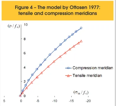
Figure 4 shows the compression and tensile meridians that are

(7)

presented by the surface given by Ottosen [22]. In the present work, however, parameters a, b, c₁, and c₂ have been determined from the relation k = f_t / f_c, using the expressions recommended by the CEB-FIP Model Code 1990 [19]:

(21)

a

= 1 / (9

k

1.4

₎

b

= 1 / (3.7

k

1.1

₎

c

1

= 1 / (0.7

k

0.9

)

c

2

= 1 – 6.8(

k

– 0.07)

2

2.4.3 Determination of peak stresses (fc1, fc2, fc3)

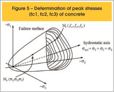
From the failure surface by Willam and Warnke [23] or from the one by Ottosen [22], the peak stresses, f_c1, f_c2, and f_c3, regarding the three directions for a determined current principal stress state (σ1, σ2, and σ3), can be found. To calculate the values of these peak

stresses, the following procedure has been used:

1. A straight line from the origin of the principal stress system to the point of current stresses M_c(σ₁, σ₂, σ₃) is determined; 2. Next, this straight line is extended until the failure surface is

reached, identifying the point M_r(f_c1, f_c2, f_c3), as can be seen in Figure 5.

The equation of the straight line that goes from the origin to the updated principal stress state (σ1, σ2, σ3) can be expressed as a

function of the octahedral stresses σ_oct and τ_oct:

(22)

0

c

oct oct c oct

oct

s

t

æ

ö

-

_ç

_÷

=

è

ø

where

3

c 1 2 3

oct

σ σ σ

σ

=

+ +

– is the updated octahedral normal stress;

(

)

2

(

) (

2

)

2

3

1 2 1 3 2 3

c oct

σ σ

τ

=

−

+

−

+

−

– is the

updated octahedral shear stress.

Numerically, the procedure is carried out by solving a system of equations that corresponds to the determination of the intersec-tion of the line, Equaintersec-tion (22), with the failure surface by Willam and Warnke [23], Equation (14), or with the failure surface by Ottosen [22], Equation (20). These calculations, in this case, were carried out by the subroutine DNEQNF, available in IMSL FORTRAN 90 MP Library [25] to solve the nonlinear system of equations. By solving the system of equations, the octahedral stresses (

σ

octr ,

r oct

τ

) at the intersection point of the line with the speciied failure surface is obtained, and with these octahe-dral stresses, the peak stresses are determined by the following expressions:

(23)

( )

2 cos

2

2 cos

3

2

2 cos

3

r r

c1 oct oct

r r

c2 oct oct

r r

c3 oct oct

f

s

t

q

p

s

t

q

p

s

t

q

=

+

æ

ö

=

+

_ç

-

_÷

è

ø

æ

ö

=

+

_ç

+

_÷

è

ø

In Figure 5, it can be noticed that the failure surface has its origin in a failure point of hydrostatic tension and opens up in the negative direction of the hydrostatic axis. Therefore, a compressive hydro-static load can not cause failure (Chen and Han [20]). With increas-ing lateral coninement, the updated stress state (σ1, σ2, σ3) gets

closer to the hydrostatic axis. In this situation, depending on the triaxial state of compression stresses, Equation (22) used to deine peak stresses could not intercept the failure surface, not allowing the determination of values for f_c1, f_c2, and f_c3. In this case, a second alternative is used for deinition of the ultimate stresses, where the octahedral normal stress, σ_oct, is considered constant, while the octahedral shear stress, τ_oct, should vary until reaching the failure surface. This procedure is similar to the previous one, only replac-ing Equation (22) by:

(24)

0

c oct oct

s

-

s

=

(8)

2.4.4 Determination of peak strains (εc1, εc2, εc3)

After determining the peak stresses, the expressions proposed by Bouzaiene and Massicotte [26] are used to calculate the peak strains, ε_c1, ε_c2, and ε_c3. These expressions are given by:

(25)

1.6

2.25

0.35

3 2

ci ci ci

ci c

c c c

f

e e

= -

é

ê

æ ö

_{ç ÷}

+

æ ö

_{ç ÷}

+

æ ö

_{ç ÷}

ù

ú

ê

è ø

ú

ë

û

_{, for}

_f

_ci

_/

_f

_c

_£

_1.

(26)

3.0

ci

2.0

ci c

c

f

e

=

e

é

_ê

æ

_ç

ö

_÷

-

ù

_ú

è

ø

ë

û

_{, for 1}

_£

_fci

_/

_fc

_£

_1.27.

(27)

5.312

ci

4.936

ci c

c

f

e

=

e

é

_ê

æ

_ç

ö

_÷

-

ù

_ú

è

ø

ë

û

_{, for fci}

_{/ fc}

_{> 1.27.}

where i = 1, 2, 3;

f_c – uniaxial compression strength of concrete;

εc – strain that corresponds to fc.

Expression (27), according to Bouzaiene and Massicotte [26], was adjusted to experimental data, respecting the continuity with Equation (26). For the directions in tension, εci = εt was considered,

where ε_t is the corresponding strain to the uniaxial tensile strength, f_t..

2.5 Control Point of Popovics-Saenz curve

It is known that concrete exhibits a softening in its stress-strain curve after peak stresses are reached. This behavior is a phe -nomenon that depends on specimens’ dimensions and shape, as well as on boundary conditions existent in the tests con -ducted. Moreover, the post-peak branch of the curve presents considerable variability, depending on test characteristics (Ba -lan et al. [14]). Therefore, to perform a realistic analysis, the definition of an appropriate model to describe the material’s post-peak behavior is essential. With Popovics-Saenz curve, an adequate estimative of concrete’s compression response can be reached by using a control point located in the post-peak branch of the equivalent uniaxial stress-strain curve. Ac -cording to Balan et al. [13], from experimental tests, the follow-ing values are proposed for the stresses and strains that define this control point:

(28)

f

fi

= 0.85 f

ci

e

_fi

= 1.41

e

_ci

(29)

f

fi

= 0.25

f

ci

e

_fi

= 4.0

e

_ci

where

f_ci – is the material strength in the i direction, with i = 1, 2, 3;

εci – is the strain that corresponds to fci.

Increases in confinement stresses in triaxial compression tests were verified to affect strength, ductility, dilatancy, and failure modes of concrete. In addition, increases in lateral confine-ments make the failure mode of concrete change from brittle to ductile (Balan et al. [14]). However, the established values in (28) and (29) define the softening surface of the material as a surface that has its shape proportionally reduced in rela-tion to the failure surface, independently of loading condirela-tions. Thus, for a better consideration of concrete’s experimental be-havior when subjected to compression, the stress values f_fi of the control point are defined as function of the peak stresses, which are dependent on the confinement stresses applied to the structure (Balan et al. [13]).

From the experimental results by Smith et al. [27], Kwon [15] defined the following coordinates for the control point:

(30)

5

4

ci fi

ci

c

fi ci

f

e

=

æ

ö

-ç

÷

è

ø

=

where, f_c is concrete’s uniaxial compression strength. As can be noticed, in this work, the above relations have also been adopted for the control point used on the deinition of the equivalent uniaxial stress-strain curve of the concrete subjected to compression.

2.6 Cracked and Crushed Concrete

In this work, a smeared crack model has been implemented, with cracks rotating according to the directions of updated principal stresses. No special treatment is given to post-peak behavior of concrete after crushing or cracking, since the equivalent uniaxial laws entirely govern the response of the material.

The criterion adopted to verify cracking or crushing occurrence was to check the equivalent uniaxial strain, in a speciic direction, to see if it is greater than the corresponding strain to the peak stress, also considering the signal of the ongoing stress.

2.7 Poisson’s ratio

The values of the Poisson’s ratios, νij, have to be determined to

(9)

compression initially decreases and, later on, increases when fail-ure is imminent. This dilatancy occurs because of the opening (or expansion) of existent microcracks in the material., Several works from the literature, like the ones published by Elwi and Murray [12], Balan et al. [13] and Kwon [15], suggest the use of an increasing function for the Poisson’s ratio to simulate that volumetric variation. In this work, the expression proposed by Kwon [15] is the one used to deine Poisson’s ratios:

(31)

i

ij ui uj

j

E

n

=

n n

where ν_ui is the Poisson’s ratio for the equivalent uniaxial direction i. The symmetry of the constitutive matrix, D_o, which was expressed in Equation (3), is guaranteed when Equation (31) is considered. For deinition of νui, the following expression is used:

(32)

1

2 3

ui ui ui

ui o i i i

vi ci ci ci

A

B

C

K

e

n n

e

é

ì

_ï

_{æ ö æ ö}

_{æ ö}

ü

_ï

ù

ê

ú

=

+

í

ç ÷ ç ÷

+

ç ÷

ý

ê

_ï

_î

_{è ø è ø}

_{è ø}

_ï

_þ

ú

ë

û

_{, with}

_i

_{= 1, 2, 3.}

where

νo – is the initial Poisson’s ratio;

1

2

i o

K

ν

=

; fi

i ci

K

_ε

ε

=

; _i ci

fi

f

K

f

σ

=

; _vi _o ci ci

K

E

f

ε

=

;

Figure 6 – Bilinear constitutive model for steel

A_i = C_i + K_i – 2; B_i = 1 – 2C_i;

(

)

(

)

2

1

i

i i

K

C

K

σ

ε ε

−

=−

−

Equation (32) is similar to the cubic expression deined by Elwi and Murray [12], which later on was used by Balan et al. [13]. Kwon [15] proposed the addition of the coeficient K_n to that cubic function to avoid Ω_c, which appears in Equation (3), to become close to zero or a negative number, since a zeroed value for Ωc would create

numer-ical problems in the inite element formulation of the constitutive law.

2.8 Implementation of the Numerical Model

for the Concrete

In this section, the determination of the stresses in the concrete is detailed. Initially, an isotropic behavior is admitted for the con -crete, considering the secant moduli of elasticity equal to the initial modulus of elasticity, i.e.,

E

₁s

=

E

₂s

=

E

₃s

=

E

_o. With these secant moduli of elasticity and the current strains for a determined load step, the total stresses are calculated, as presented in Table 1. With these total stresses related to the global system of ref-erence, the current principal stresses, σ₁, σ₂, σ₃, are determined. From these principal stresses, the equivalent uniaxial strains for the three principal directions are determined.

With the principal stresses and the failure surface chosen for the concrete, the peak values of stresses and strains are also deter-mined, as explained in 2.4.3 and 2.4.4. Next, the stresses and strains of the control point used in the descending branch of the Popovics-Saenzcurve [Equation (11)] are also obtained. The new equivalent uniaxial stress-strain curves are deined for the three directions of principal stresses with the determination of these vari-ables. From these three equivalent uniaxial curves, the new values of the current principal stresses are calculated.

Finally, from the principal stresses, the total stresses related to the glob -al system of reference are updated. In an iterative process, -all the de-scribed steps are repeated until convergence, as indicated in Table 1.

3. Constitutive model for the steel

Since reinforcing bars resist to forces that primarily develop along their axial direction, i.e., perpendicular forces to rebars’ axes can be neglected, it is enough to know rebars’ properties relatively to an uniaxial stress state.

The shape of the stress-strain diagram for steel can be represented by four branches: an elastic branch; a yielding branch; a hardening branch; and a softening branch. In the literature, however, there are several simpliied representations for that uniaxial stress-strain be-havior: elastic-perfectly plastic model; elastic-linear work hardening model; trilinear approximation; and a complete stress-strain curve. In this work, a bilinear diagram with work hardening was adopted for the monotonic stress-strain curve, as deined in Figure 6 and by:

(33)

s

_s

=

e

_s

_E

_so

if

|e

_s

|

<

e

_y

s

_s

= +

f

y

+ (

e

s

–

e

y

)

E

s1

if

e

y

£

e

s

£

e

su

(10)

where

εsu – is the strain which corresponds to the ultimate stress, fsu, of

the steel;

σs, εs – are the stress and strain in the reinforcing bar;

f_y, ε_y – are the yielding stress and strain;

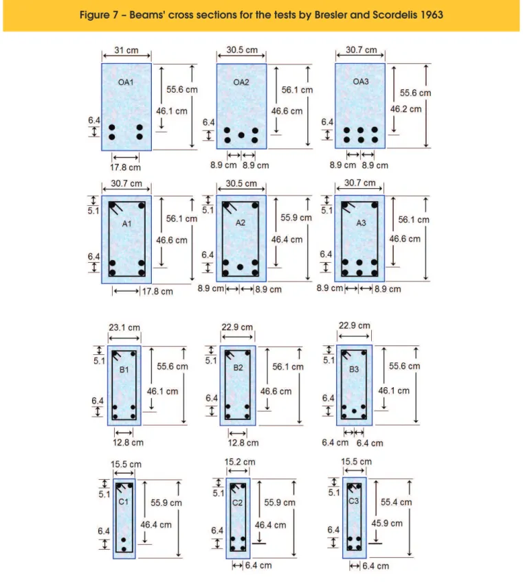
Figure 7 – Beams' cross sections for the tests by Bresler and Scordelis 1963

E_so – is the initial modulus of elasticity;

(11)

4. Numerical Application

In this section, the results obtained with the computational model developed are compared with values determined ex-perimentally for reinforced concrete beams. These experi -mental results were presented by Bresler and Scordelis [28], concerning twelve beams in reinforced concrete primarily subjected to shear.

The twelve beams were arranged in four series of three units, with each series concerning a different quantity of longitudinal reinforcement, quantity of stirrups, span length, cross-section-al dimensions, and concrete’s strength. All beams had rectan-gular cross-sections and their details can be seen in Figure 7, with additional information presented in Tables 2 and 3. All bottom longitudinal bars were 28.7 mm in diameter, while bars of 12.7 mm were used at the top of the beams, and, when present, stirrups were made of 6.4 mm bars. One of the series had no stirrups at all, and was labeled as OA series. All beams

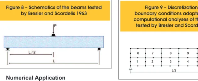
Figure 8 – Schematics of the beams tested

by Bresler and Scordelis 1963

boundary conditions adopted for the

Figure 9 – Discretization and

computational analyses of the beams

tested by Bresler and Scordelis 1963

Figure 10 – Load-deflection curves for the tests by Bresler and Scordelis 1963: Series 1

were subjected to monotonic concentrated loads applied at midspan, as illustrated in Figure 8.

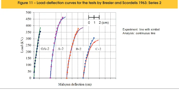
For the computational analysis, a finite element discretization of ten quadratic hexahedral elements was adopted to model the beams. Taking advantage of the problem’s symmetry, the discretization and boundary conditions were the ones shown in Figure 9. Load-displacement curves, as presented in Figures 10 to 12, were used for validation of the numerical analysis. In Table 4, the failure loads obtained with the numerical program are presented and can be compared with the experimental re -sults also indicated.

(12)

Figure 11 – Load-deflection curves for the tests by Bresler and Scordelis 1963: Series 2

Figure 12 – Load-deflection curves for the tests by Bresler and Scordelis 1963: Series 3

5. Conclusions

This work presents a general formulation for nonlinear analyses through inite elements of reinforced concrete structures. The con-stitutive law used for concrete is orthotropic with its axes parallel to the updated principal stresses’ directions. The model also uses the concept of equivalent uniaxial strain; a concept originally

(13)

The models were implemented in a inite element program origi -nally developed by Hinton [29] and, in order to consider reinforcing bars in it, the embedded reinforcement model proposed by Elwi and Hrudey [10] was used after its extension to the 3D case. A uniaxial constitutive model with bilinear elastic with work-hardening was implemented to represent steel’s stress-strain curve. Moreover, comparisons made between the predictions given by the numerical model with experimental data showed an excellent agreement.

6. References

[01] Patrick, M.D. and Sharon Huo, X. Finite element modeling of slab-on-beam concrete bridge

superstructures. Computers and Concrete, v.1, n.3, p.355-369, 2004.

[02] Kim, S.H. and Aboutaha, R.S. Finite element analysis of carbon iber-reinforced polymer (CFRP)

strengthened reinforced concrete beams. Computers and Concrete, v.1, n.4, p.401-416, 2004.

[03] Park, S. and Aboutaha, R. Finite element modeling methodologies for FRP strengthened RC

members. Computers and Concrete, v.2, n.5, p.389-409, 2005.

[04] Hoque, M., Rattanawangcharoen, N. and Shah, A.H. 3D nonlinear mixed inite-element analysis of RC beams and plates with and without FRP reinforcement. Computers and Concrete, v.4, n.2, p.135-156, 2007.

[05] Smadi, M.M. and Belakhdar, K.A. Nonlinear inite element analysis of high strength concrete slabs. Computers and Concrete, v.4, n.3, p.187-206, 2007. [06] Souza, R.A., Kuchma, D.A., Park, J.W. and

Bittencourt, T.N. Nonlinear inite element analysis of four-pile caps supporting columns subjected to generic loading. Computers and Concrete, v.4, n.5, p.363-376, 2007.

[07] Shayanfar, M.A. and Saiey, A. Hypoelastic modeling of reinforced concrete walls. Computers and Concrete, v.5, n.3, p.195-216, 2008.

[08] Manzoli, O.L., Oliver, J., Huespe, A.E. and Diaz, G. A mixture theory based method for three-dimensional modeling of reinforced concrete members with embedded crack inite elements. Computers and Concrete, v.5, n.4, p.401-416, 2008.

[09] Bono, G.F.F. Constitutive models for tridimensional analysis or reinforced concrete structures through the Finite Element Method. PhD Dissertation, Federal University of Rio Grande do Sul, Brazil, 2008. [10] Elwi, A.E. and Hrudey, M. Finite element model for

curved embedded reinforcement. ASCE J. Eng. Mech., v.115, n.4, p.740-754, 1989.

[11] Darwin, D. and Pecknold D.A. Nonlinear biaxial stress–strain law for concrete. ASCE J. Eng. Mech., v.103, n.2, p.229–241, 1977.

[12] Elwi, A.A. and Murray D.W. A 3D hypoelastic

concrete constitutive relationship. ASCE J. Eng. Mech. Div., v.105(EM4), p.623-641, 1979.

[13] Balan, T.A., Filippou, F.C. and Popov E.P. Constitutive model for 3D cyclic analysis of concrete structures.

ASCE J. Eng. Mech., v.123, n.2, p.143-153, 1997. [14] Balan, T.A., Spacone, E. and Kwon, M. A 3D

hypoplastic model for cyclic analysis of concrete structures. Eng. Struct., v. 23, n.4, p.333–342, 2001. [15] Kwon, M. Three dimensional inite element analysis for reinforced concrete members. PhD dissertation, Department of Civil, Environmental, and Architectural Engineering, University of Colorado, Boulder, 2000. [16] Kwon, M. and Spacone, E. Three-dimensional inite

element analyses of reinforced concrete columns. Computers and Structures, v.80, p.199-212, 2002. [17] Saenz I. P. Discussion of equation for the stress–strain

curve of concrete by P. Desay and S. Krishnan. ACI J., v.61, n.9, p.1229–1235, 1964.

[18] Popovics, S. Numerical approach to the complete stress–strain relation for concrete. Cement Concr. Res., v.3, n.5, p.583–599, 1973.

[19] Comitê Euro-International du Béton. CEB-FIP Model code 1990. Thomas Telford Services Ltda, 1993. [20] Chen, W.F. and Han, D.J. Plasticity for Structural

Engineers, Springer-Verlag New York Inc., New York, 1988.

[21] Menetrey, P. and Willam, K.J. Triaxial failure criterion for concrete and its generalization. ACI Struct. J., v. 92, n.3, p.311–318, 1995.

[22] Ottosen, N.S. A failure criterion for concrete. ASCE J. Eng. Mech. Div., v.103(EM4), p.527-627, 1977. [23] Willam, K.J and Warnke, E.P. Constitute models for

the triaxial behavior of concrete. Int. Assoc. Bridge Struct. Proc., v.19, p.1–30, 1974.

[24] Kupfer, H.B., Hilsdorf H.K. and Rusch, H. Behavior of concrete under biaxial stress. ACI J., v.66, n.8, p.656-666, 1969.

[25] IMSL Fortran 90 MP Library. Fortran 90 Subroutines and Functions, Ed. 6.5, 2000.

[26] Bouzaiene, A. and Massicotte, B. Hypoelastic tridimensional model for nonproportional loading of plain concrete”, ASCE J. Eng. Mech., v.123, n.11, p.1111-1120, 1997.

[27] Smith, S.S., Willam, K.J., Gerstle, K.H. and Sture, S. Concrete over the top, or: is there life after peak?. ACI J., v.86, n.5, p.491–497, 1989.

[28] Bresler, B. and Scordelis, A.C. Shear strength of reinforced concrete beams. ACI J., v.60, n.1, p.51-72, 1963.