Paulo B. Gonçalves
and Frederico M. A. da Silva
Pontifical University of Rio de Janeiro - PUC – Rio Civil Engineering Department 22453-900 Rio de Janeiro, RJ. Brazil [email protected]Zenon J. G. N. del Prado
Federal University of Goiás Civil Engineering Department Praça Universitaria 74605-200 Goiânia, GO. Brazil. [email protected]Transient Stability of Empty and
Fluid-Filled Cylindrical Shells
In the present work a qualitatively accurate low dimensional model is used to study the non-linear dynamic behavior of shallow cylindrical shells under axial loading. The dynamic version of the Donnell non-linear shallow shell equations are discretized by the Galerkin method. The shell is considered to be initially at rest, in a position corresponding to a pre-buckling configuration. Then, a harmonic excitation is applied and conditions to escape from this configuration are sought. By defining steady state and transient stability boundaries, frequency regimes of instability may be identified such that they may be avoided in design. Initially a steady state analysis is performed; resonance response curves in the forcing plane are presented and the main instabilities are identified. Finally, the global transient response of the system is investigated in order to quantify the degree of safety of the shell in the presence of small perturbations. Since the initial conditions, or even the shell parameters, may vary widely, and indeed are often unknown, attention is given to all possible transient motions. As parameters are varied, transient basins of attraction can undergo quantitative and qualitative changes; hence a stability analysis which only considers the steady-state and neglects this global transient behavior, may be seriously non-conservative.
Keywords: Cylindrical shells, fluid-structure interaction, parametric instability, nonlinear vibrations
Introduction
Thin-walled cylindrical shells are widely used in many industries. Due to the increasing use of high-strength materials, sophisticated numerical techniques and optimization methods in analysis, the design of such shells is often buckling-critical. In many circumstances these shells are subjected not only to static loads but also to dynamic disturbances and filled with internal fluid. However, thin-walled cylindrical shells when subjected to axial compressive loads often exhibit a highly nonlinear behavior with a high imperfection sensitivity and may loose stability at loads levels as low as a fraction of the material strength.1
Many studies are concerned with the analysis of shells vibrating in vacuum; far fewer are focused on the analysis of the nonlinear vibrations of cylindrical shells in contact with a dense fluid. One of the first studies on vibrations of circular cylindrical shells in contact with a dense fluid considering shell nonlinearity is due to Ramachandran (1979). He studied the large-amplitude vibrations of circular cylindrical shells having circumferentially varying thickness and immersed in a quiescent, non-viscous and incompressible fluid, using the Donnell’s shell theory.
Boyarshina (1984, 1988) studied theoretically the nonlinear free and forced vibrations and stability of a circular cylindrical tank partially filled with a liquid and having a free surface. Here, nonlinearity is attributed to the interaction of free surface waves and elastic flexural vibrations of the shell.
Gonçalves and Batista (1988) considered simply supported circular cylindrical shells filled with incompressible fluid. To model the shell, Sanders’ nonlinear shell theory and a novel mode expansion that includes two terms in the radial direction (the asymmetric and the axisymmetric ones) and ten terms to describe the in-plane displacements were used. Numerical results were obtained concerning the effect of the liquid on the nonlinear behavior of shells. It was found that the presence of a dense fluid increases the softening characteristics of the frequency-amplitude
Presented at XI DINAME – International Symposium on Dynamic Problems of Mechanics, February 28th - March 4th, 2005, Ouro Preto. MG. Brazil. Paper accepted: June, 2005. Technical Editor: José Roberto de França Arruda.
relation when compared with the results for the same shell in vacuum.
Chiba (1993) studied experimentally large-amplitude vibrations of two vertical cantilevered circular cylindrical shells made of polyester sheets partially filled with water to different levels. He observed that for bulging modes with the same axial wave number, the weakest degree of softening nonlinearity can be attributed to the mode having the minimum natural frequency, as observed for the same empty shells. He also found that shorter tanks have a larger softening nonlinearity than taller ones, as in vacuum. The tank with a lower liquid height has a stronger softening nonlinearity than the same tank with a higher liquid level. Traveling wave modes and coupling between two bulging modes (and between two sloshing modes) were also observed.
Amabili et al (1998) studied the nonlinear free and forced vibrations of a simply supported, circular cylindrical shell in contact with an incompressible and non-viscous, quiescent dense fluid. Donnell’s nonlinear shallow-shell theory is used, so that moderately large vibrations can be analyzed. The boundary conditions on radial displacement and continuity of circumferential displacement are exactly satisfied, while the axial constraint is satisfied “on the average”. The problem is reduced to a system of ordinary differential equations by means of the Galerkin method, assuming an appropriate deflection shape. The mode shape is expanded by using two asymmetric modes (driven and companion modes) plus the axisymmetric mode.
In the present study, a low dimensional model which retains the essential nonlinear terms is used to study the nonlinear oscillations and instabilities of the shell. Here the interest is focused on a pivotal interaction between non-symmetric and axisymmetric modes which allows the escape from the pre-buckling configuration. To discretize the shell, Donnell shallow shell equations, modified with the transverse inertia force, are used together with Galerkin method to derive a set of coupled ordinary differential equations of motion. These equations are integrated numerically using the fourth order Runge-Kutta method. In order to study the nonlinear behavior of the shell, several numerical strategies were used to obtain time responses, Poincaré maps and bifurcation diagrams. The interested reader will find a description of the relevant numerical algorithms in Del Prado (2001).
potencial. The solution for the velocity potencial is taken as a sum of suitable functions, where the unknown parameters are determined by the kinetic condition along the shell wetted surface (Batista and Gonçalves, 1988).
Steady state and transient stability boundaries are presented and special attention is devoted to the determination of the critical load conditions. From this theoretical analysis, dynamic buckling criteria can be property established which may constitute a consistent and rational basis for design of these shell structures under harmonic loading.
Problem Formulation
Shell Equations
Consider a perfect thin-walled fluid-filled circular cylindrical shell of radius R, length L, and thickness h. The shell is assumed to be made of an elastic, homogeneous, and isotropic material with Young’s modulus E, Poisson ratio ν, and mass per unit area M. The axial, circumferential and radial co-ordinates are denoted by, respectively, x, y and z, and the corresponding displacements on the shell surface are in turn denoted by U, V, and W, as shown in Fig. 1.
Figure 1. Shell geometry and coordinate system.
The shell is subjected to a uniformly distributed axial load given by:
( )
t P P( )
tP = 0+ 1cosω (1)
where P0 is the uniform static load applied along the edges x=0, L,
P1 is the magnitude of the harmonic load, t is time and ω is the forcing frequency.
The nonlinear equations of motion based on the Von Karmán-Donnell shallow shell theory, in terms of a stress function f and the transversal displacement w are given by:
xy , xy , yy , xx , xx , yy , h w F R w F w F R p w w w M 2 1 4 2 1 − + + + = ∇ + +β ɺ β
ɺ ɺ (2) 2 , , , , 4 1 1 xy yy xx
xx w w w
w R f h
E ∇ =− − + (3)
where: 2 0 2 1 y P f f f
F= F+ F=−
and ph is the fluid pressure, ∇4 is the biharmonic operator, β1 and β2 are damping coefficients and D is the flexural rigidity defined as:
(
2)
3 1 12 v h E D − = (4)
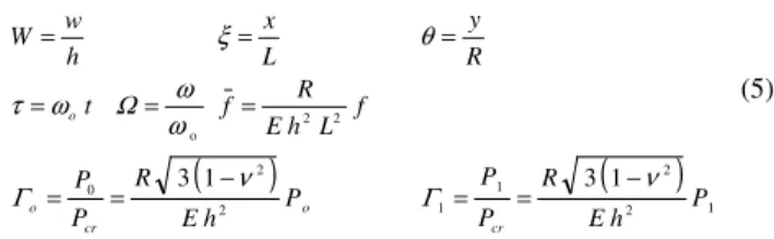
In the foregoing, the following non-dimensional parameters will be introduced:
(
)
(
)
1 2 2 1 1 2 2 0 2 2 o 1 3 1 3 P h E R P P P h E R P P f L h E R f t R y L x h w W cr o cr o o ν Γ ν Γ ωω Ω ω τ θ ξ − = = − = = = = = = = = (5)where ωo is the lowest natural frequency of the empty shell.
Modal Analysis
The numerical model is developed by expanding the transversal displacement component w in series in the circumferential and axial variables. From previous investigations on modal solutions for the non-linear analysis of cylindrical shells under axial loads (Hunt et al. 1986; Gonçalves and Batista, 1988; Gonçalves and Del Prado, 2002) it is observed that, in order to obtain a consistent modeling with a limited number of modes, the sum of shape functions for the displacements must express the non-linear coupling between the modes and describe consistently the unstable post-buckling response of the shell as well as the correct frequency-amplitude relation.
The dimensionless lateral deflection W can be generally described as (Gonçalves and Batista, 1988):
( ) (
)
(
θ) (
πξ)
ξ π θ m l sin n k cos W m j sin n i cos W W ij , , l , , k ij , , j , , i
∑
∑
∑
∑
= = = = + = 4 2 0 4 2 0 5 3 1 5 3 1 (6)where n is the number of waves in the circumferential direction of the basic buckling or vibration mode, m is the number of half-waves in the axial direction, θ = y / R and ξ = x / L.
These modes represent both the symmetric and asymmetric components of the shell deflection pattern. The first double series represents the unsymmetrical modes with odd multiples of the basic wave numbers m and n. The second double series represents, besides the asymmetric modes which contains an even multiple of the basic wave numbers m and n and rosette modes, the axysimmetric modes which play an important role in the non-linear modal coupling and loss of stability of the shell.
Previous studies on buckling of cylindrical shells have shown that the most important modes are the basic buckling or vibration mode and the axi-symmetric mode with twice the number of half waves in the axial direction as the basic mode, that is:
( )
( ) (
)
( )
τ(
πξ)
ζ ξ π θ τ ζ m cos m sen n cos W 2 02 11 + = (7)
potential barrier connected with the unstable equilibrium positions lying on the initial post-buckling path.
Substituting the assumed form of the lateral deflection, Eq. (7), on the right-hand side of the compatibility Eq. (3), this equation can be solved to obtain the stress function f in terms of w together with the relevant boundary and continuity conditions. Upon substituting the modal expressions for f and w into Eq. (2) and applying the Galerkin method, a set of non-linear ordinary differential equations is obtained in terms of modal amplitudes ζ(τ)ij.
Fluid Mechanics Equations
The shell is assumed to be completely fluid-filled. The irrotational motion of an incompressible and non-viscous fluid can be described by a velocity potential φ(x, r, θ, t). This potential function must satisfy the Laplace equation which can be written in dimensionless form as:
0 1
1
, , 2 ,
,ξξ+ κ+ φθθ+φκκ=
κ φ κ
φ (8)
where:
R r =
κ φ =γφ R2 [ R2(1 2)/E]1/2
s ν
ρ
γ= −
The dynamic fluid pressure acting on the shell surface is obtained from the Bernoulli equation:
t , S
F h
p φ
δ γ ρ ρ
−
= 2
4 (9)
where ρF is the density of the fluid and ρS is the shell material density.
At the shell-fluid interface, the fluid velocity normal to the shell surface must be equal to the shell velocity in this direction, that is:
(
∂w ∂t)
=2 /
, γδ
φκ (10)
where δ=h/2R.
Further, for a fluid-filled shell, the following restriction must be imposed at κ = 0:
0
,κ =
φ (11)
Solving equations (8) to (11), one obtains the following expressions for the hidrodynamic fluid pressure:
ph=ζ11,ττmacos
( ) (
nθ sin mπξ)
(12)where ma is the added mass due to the fluid contained in the shell, which is given by:
(
)
1(
(
)
)
1− −
− =
ξ π ξ π
ξ π ξ
π ρ
m n m
I m I m R m
n n F
a (13)
where In-1 and In are Bessel functions.
Results
To check the validity and accuracy of the present methodology for the determination of the natural frequencies, a key point in any non-linear dynamic analysis, empty and fluid-filled cylindrical
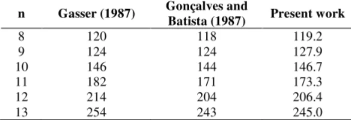
shells are analyzed and the results are compared with experimental and other numerical values found in literature. As a first example, the lowest natural frequencies of a simply supported empty cylinder are compared with the analytical solution derived by Dym (1973) using Sanders’ shell theory and the experimental results obtained by Gasser (1987). The results are shown in Table 1. For the same shell, the present results for a water filled shell are compared with those obtained experimentally by Gasser (1987) and the numerical results obtained by Gonçalves and Batista (1987) in Table 2. In both cases, there is an excellent agreement between all results.
Table 1. Comparison of natural frequencies (Hz) for an empty cylindrical shell.(m = 1, L = 0.41 m, R = 0.3015 m, h = 0.001 m, E = 2.1x10⁸
kN/m²,
νννν = 0.3, ρρρρ = 7850 kg/m³).
n Gasser (1987) Dym (1973) Present work
7 318 305.32 303.35
8 278 281.37 280.94
9 290 288.28 288.71
10 334 317.51 318.40
11 362 362.22 363.33
12 418 417.96 419.19
13 478 482.23 483.51
14 550 553.67 554.97
Table 2. Comparison of natural frequencies (Hz) for a cylinder filled with water. (m = 1, L = 0.41 m, R = 0.3015 m, h = 0.001 m, E = 2.1x10⁸
kN/m²,
νννν = 0.3, ρρρρ = 7850 kg/m³, ρρρρF = 1000 kg/m³).
n Gasser (1987) Gonçalves and
Batista (1987) Present work
8 120 118 119.2
9 124 124 127.9
10 146 144 146.7
11 182 171 173.3
12 214 204 206.4
13 254 243 245.0
Consider a thin-walled cylindrical shell with h=0.002m, R=0.2 m, L=0.4 m, E=2.1x10⁸kN/m2, ν=0.3, β1=2εMω0, with ε=0.003 (fluid-filled shell) and ε=0.0008 (empty shell) (Popov et al. 1998), and β2=ηD with η=0.0001. The shell and fluid densities are:
ρs=7850kg/m3 and ρF=1000kg/m3. For this shell geometry the lowest natural frequency occurs for (n ,m)=(5, 1).
Now the parametric instability and escape from the pre-buckling configuration of the fluid-filled cylinder under axial harmonic forcing, as described by Eq. (1), will be considered. In the following, the constant part of the loading (Γ0) is assumed to be between the upper and lower static critical load of the shell. In these circumstances, the shell potential energy exhibits three wells, one associated with the fundamental pre-buckling configuration and two wells associated with the two possible post-buckling configurations. If the cylinder is subjected to a periodic axial load, it will undergo the familiar longitudinal forced vibration, exhibiting a uniform transversal motion, due to the effect of Poisson’s ratio, also known as breathing mode. However, at certain critical values, the longitudinal motion becomes unstable and the cylinder executes transverse bending vibrations.
control parameter Γ1 is increased beyond a critical value, the shell exhibits initially an exponential growth of the amplitude, as shown in Fig. 2.b, converging to a limit cycle within the pre-buckling well. In this case, the trivial solution becomes unstable (parametric instability) and the system converges to a period-two stable solution. If Γ1 is increased to a higher value, for example Γ1=1.30, the shell escapes from the pre-buckling well (snap-through buckling) and exhibits large cross-well chaotic motions, as shown in Fig. 2.c, or small amplitude oscillation around a post-buckling configuration.
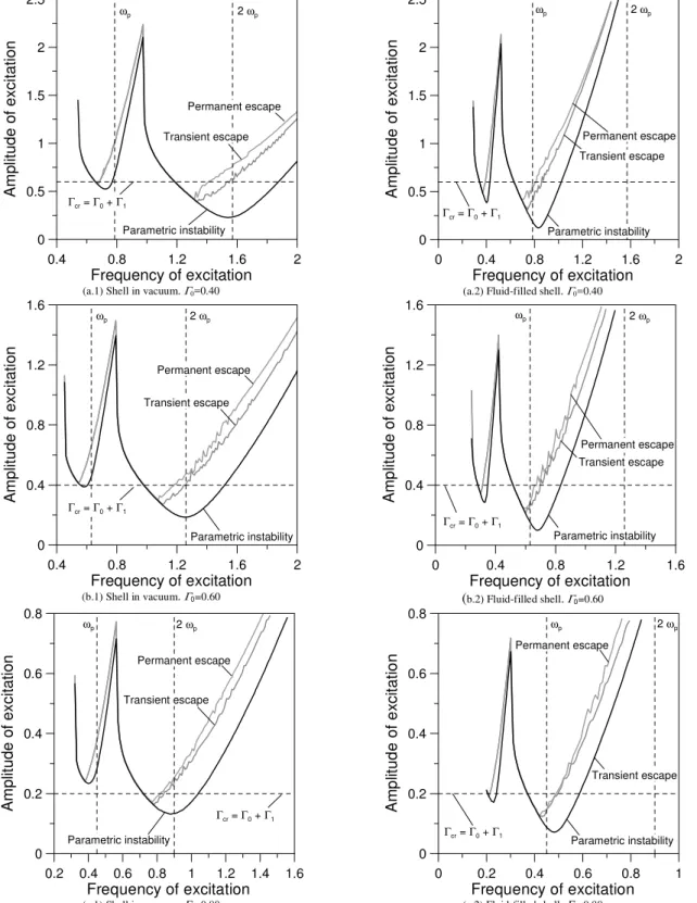
Figure 3 shows the numerically obtained parametric instability boundary as well as the transient and permanent escape boundaries for the fluid-filled shell and the same shell in vacuum, in (frequency of excitation x amplitude of excitation) control space for Γ0=0.40,
Γ0 =0.60 and Γ0=0.80. The lower stability boundary corresponds to parameter values for which small perturbations from the trivial solution will result in an initial growth in the oscillations; therefore it defines the parametric instability boundary. The second limit corresponds to escape from the pre-buckling potential well in a slowly evolving environment. These curves were obtained by increasing slowly the amplitude while holding the frequency constant. As one can observe, the parametric stability boundary is composed of various “curves”, each one associated with a particular bifurcation event. The deepest well is associated with the principal instability region at ω=2ωp, while the second well to the left is the
secondary instability region occurring around ω=ωp and the other smaller wells to the left are connected with super-harmonic resonances. The horizontal dotted line corresponds to the static critical load of this shell. Comparing Figures 3.a, 3.b and 3.c, one can conclude that the static pre-loading has the effect of lowering the stability boundaries, of enlarging the width of the instability regions and of shifting the instability regions to the left. In both cases the instability boundaries can be much lower than the static critical load. The fluid has a similar influence on the stability boundaries. This is expected since the influence of the fluid is to increase the effective mass of the system, decreasing consequently the natural frequencies.
For the region between the parametric instability limit and the transient escape limit, the shell exhibits vibrations in the pre-buckling potential well during both permanent and transient states. When comparing the permanent and transient boundaries, one can observe that the transient escape limit is lower than the permanent one. This means that the shell may exhibit large amplitude vibrations during the transient state but converge to a low amplitude solution within the pre-buckling well when the steady-state response is reached. A structure may display in a nonlinear regime long transients, but their lengths can not be known a priori. So, in order to avoid any damage due to large amplitude vibrations the transient response of the shell must be analyzed in detail.
0 200 400 600
Time
-0.04 -0.02 0 0.02 0.04
ζ11
-0.04 -0.02 0 0.02 0.04
ζ11
-0.02 -0.01 0 0.01 0.02
d
ζ11
/d
t
-1 0 1
ζ11 -1
0 1
d
ζ11
/d
t
(a) Γ1=0.45
0 200 400 600
Time
-4 -2 0 2 4
ζ11
-4 -2 0 2 4
ζ11 -1.5
-1 -0.5 0 0.5 1 1.5
d
ζ11
/d
t
-0.3 -0.2 -0.1 0 0.1 0.2 0.3
ζ11 -1.5
-1 -0.5 0 0.5 1 1.5
d
ζ11
/d
t
(b) Γ1=0.80
0 200 400 600
Time
-20 -10 0 10 20
ζ11
-15 -10 -5 0 5 10 15
ζ11 -8
-4 0 4 8
d
ζ11
/d
t
-15 -10 -5 0 5 10 15
ζ11 -0.6
-0.4 -0.2 0 0.2 0.4 0.6
d
ζ11
/d
t
(c) Γ1=1.30
0.4 0.8 1.2 1.6 2
Frequency of excitation
0 0.5 1 1.5 2 2.5
A
m
p
lit
u
d
e
o
f
e
x
c
it
a
ti
o
n
Parametric instability
Permanent escape
Transient escape 2 ωp
ωp
Γcr = Γ0 + Γ1
(a.1) Shell in vacuum. Γ0=0.40
0 0.4 0.8 1.2 1.6 2
Frequency of excitation
0 0.5 1 1.5 2 2.5
A
m
p
lit
u
d
e
o
f
e
x
c
it
a
ti
o
n
Parametric instability Permanent escape Transient escape
2 ωp
ωp
Γcr = Γ0 + Γ1
(a.2) Fluid-filled shell. Γ0=0.40
0.4 0.8 1.2 1.6 2
Frequency of excitation
0 0.4 0.8 1.2 1.6
A
m
p
lit
u
d
e
o
f
e
x
c
it
a
ti
o
n
Parametric instability Permanent escape
Transient escape 2 ωp
ωp
Γcr = Γ0 + Γ1
(b.1) Shell in vacuum. Γ0=0.60
0 0.4 0.8 1.2 1.6
Frequency of excitation
0 0.4 0.8 1.2 1.6
A
m
p
lit
u
d
e
o
f
e
x
c
it
a
ti
o
n
Parametric instability Permanent escape Transient escape
2 ωp
ωp
Γcr = Γ0 + Γ1
(b.2) Fluid-filled shell. Γ0=0.60
0.2 0.4 0.6 0.8 1 1.2 1.4 1.6
Frequency of excitation
0 0.2 0.4 0.6 0.8
A
m
p
lit
u
d
e
o
f
e
x
c
it
a
ti
o
n
Parametric instability
Permanent escape
Transient escape 2 ωp
ωp
Γcr = Γ0 + Γ1
(c.1) Shell in vacuum. Γ0=0.80
0 0.2 0.4 0.6 0.8 1
Frequency of excitation
0 0.2 0.4 0.6 0.8
A
m
p
lit
u
d
e
o
f
e
x
c
it
a
ti
o
n
Parametric instability Permanent escape
Transient escape 2 ωp
ωp
Γcr = Γ0 + Γ1
(c.2) Fluid-filled shell. Γ0=0.80
Figure 3. Instability boundaries in control space for different values of static load.
Figure 4 shows typical bifurcation diagrams connected with the principal instability region for the fluid-filled shell as a function of the forcing amplitude Γ1, for different values of the forcing frequency Ω. These bifurcation diagrams where obtained by numerical continuation techniques (Del Prado, 2001). In these diagrams a dotted line means unstable solutions and a continuous
configuration. Also, the 2T solution exhibits a stable branch between two unstable branches. So, for load levels lower than the critical value the shell may display different types of behavior within the pre-buckling well. As observed in Fig. 4.a, this non-trivial stable region corresponds to forcing values lower than the critical load. This leaves a regime where there is no attractor within the
pre-buckling well after the critical point is reached and hence an unavoidable jump to escape under increasing forcing occurs. This explains why in this region the numerically obtained parametric instability boundary practically coincides with the transient and permanent escape boundaries.
0 0.2 0.4 0.6 0.8
Amplitude of excitation
-3 -2 -1 0 1 2 3
ζ11
0 0.2 0.4 0.6 0.8
Amplitude of excitation
-1.5 -1 -0.5 0 0.5 1 1.5
ζ11
0 0.4 0.8 1.2
Amplitude of excitation
-0.4 -0.2 0 0.2 0.4
ζ11
(a) Ω=0.60 (b) Ω=0.78 (c) Ω=1.00
Figure 4. Bifurcation diagrams of the Poincaré map. Principal instability region for fluid-filled shell, ΓΓΓΓ0=0.40.
(a) Γ1=0.40 (b) Γ1=0.60
(c) Γ1=0.80 (d) Γ1=1.10
Figure 5. Cross sections of the basins of attraction, in transient state, for increasing values of the forcing amplitude ΓΓΓΓ1 of the fluid-filled cylindrical shell.
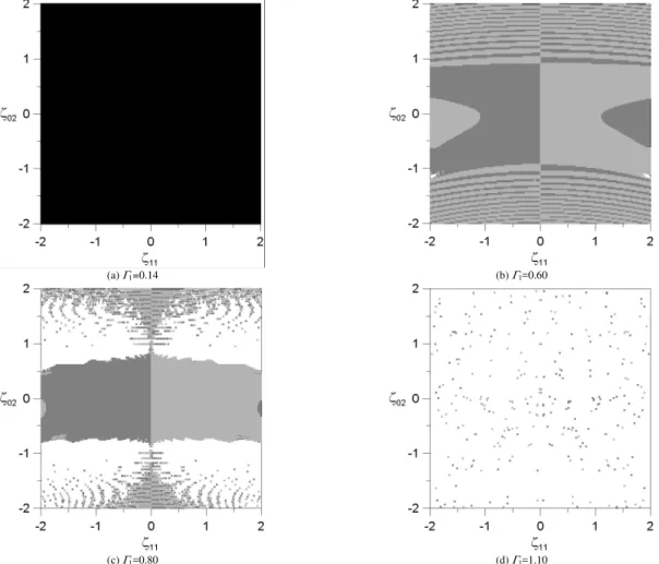
(a) Γ1=0.14 (b) Γ1=0.60
(c) Γ1=0.80 (d) Γ1=1.10
Figure 6. Cross sections of the basins of attraction, in permanent state, for increasing values of the forcing amplitude ΓΓΓΓ1of the fluid-filled cylindrical shell. Evolution of the basin forΓΓΓΓ0=0.40 andΩΩΩΩ=1.00. Parametric instability load=0.525.
In Figure 4.b, the jump is indeterminate. The bifurcation is sub-critical, but the stable small-amplitude non-trivial solution subsists for forcing values higher than the critical load. So, when the fundamental trivial solution becomes unstable, the response may re-stabilize within the pre-buckling well or jump to a remote attractor. The response that is attained physically depends on the initial conditions. The bifurcation diagram shown in Fig. 4.c is typical of the right ascending branch of the stability boundary. When Γ1 is lower than the critical value, the only possible steady state solution within the pre-buckling well is the trivial one, which is stable. Consequently, the response is trivial. When Γ1 is greater than a critical value, there are two possible steady state solutions: (a) the trivial one, which is unstable; and (b) a finite amplitude period-two (2T) solution, which is stable. In this case, since disturbances are always present, the response is non-trivial. Also, these figures show that as Γ1 increases from zero, the response consists of the trivial solution. As Γ1 exceeds the critical value, ζ11 begins to increase slowly with increasing Γ1. The critical value in this case is a supercritical bifurcation. As the amplitude of the forcing increases, the amplitude of the response increases until the escape boundary is reached. Before escape occurs, the period-two solution may also become unstable, being followed by a period doubling cascade, eventually reaching a narrow zone of chaotic motion.
In order to evaluate the safety of the structure one should analyze the behavior of the basins of attraction of the solutions in both transient and permanent states. Figure 5 shows the evolution of the transient basin of attraction for increasing values of the forcing
amplitude Γ1, Ω=1.00 and Γ0=0.40. Here the ζ11×ζ02 cross-sections of the four dimensional phase space
(
ζɺ11=ζɺ02=0.0)
are shown for increasing values of the forcing amplitude. Figure 6 shows the evolution of the permanent basin of attraction for increasing values of the forcing amplitude Γ1, Ω=1.00 and Γ0=0.40. Both figures are associated with the bifurcation diagram of Fig. 4.c and cover the same set of initial conditions.In Figure 5 the gray area is associated with the escape during the transient response and the white area corresponds to the fundamental trivial and period-two stable solutions within the pre-buckling well. As Γ1 increases the region associated with the escape increases and after a certain critical value, it covers completely the analyzed region, showing that escape occurs for any set of initial conditions during the transient response, well before the critical escape load displayed in the bifurcation diagram of Fig. 4.c is reached.
decreases and a rapid erosion is observed. Also, after a certain critical value the whole basin of attraction becomes fractal. In this case the response becomes very sensitive to the initial conditions and the steady state response, unpredictable.
Comparing the trivial and period-two areas of Fig. 5 and Fig. 6, one can observe that the basin area occupied by the transient response is smaller than the area occupied by the permanent response. So, a practical design criterion must be based on the transient analysis rather than on the steady state response of the system. Also, the critical loads obtained from the bifurcation diagrams are not enough to evaluate the robustness of the structure in the presence of unavoidable disturbances occurring during its construction or service life. The analysis of size and structure of the basin of attraction must be taken into account in order to specify allowable disturbances in a dynamic environment. A detailed parametric analysis of the basin evolution considering empty and fluid-filled shells can be found in Silva (2004).
Concluding Remarks
Based on Donnell’s shallow shell equations, an accurate low-dimensional model is derived and applied to the study of the nonlinear vibrations of an axially loaded fluid-filled circular cylindrical shell in transient and permanent states. The results show the influence of the modal coupling on the post-buckling response and on the nonlinear dynamic behavior of fluid-filled circular cylindrical shells. Also the influence of a static compressive loading on the dynamic characteristics is investigated with emphasis on the parametric instability and escape from the pre-buckling configuration. The most dangerous region in parameter space is obtained and the triggering mechanisms associated with the stability boundaries are identified. Also the evolution of transient and permanent basin boundaries is analyzed in detail and their importance in evaluating the degree of safety of a structural system is discussed. It is shown that critical bifurcation loads and permanent basins do not offer enough information for design. Only a detailed analysis of the transient response can lead to safe lower bounds of escape (dynamic buckling) loads in the design of fluid-filled cylindrical shells under axial time- dependent loads.
Acknowledgements
This work was made possible by the financial support of the Brazilian Research Council – CNPq.
References
Amabili, M., Pellicano, F. and Païdoussiss, M., 1998, “Nonlinear Vibrations of Simply Supported Circular Cylindrical Shells, Coupled to Quiescente Fluid”, Journal of Fluids and Structures, Vol. 12, pp. 883-918.
Amabili, M., Pellicano, F. and Païdoussis, M. P., 2000, “Nonlinear vibrations of fluid-filled, simply supported circular cylindrical shells: theory and experiments”, Nonlinear Dynamics Plates and Shells; AMD, . New York: ASME, Vol. 238, pp. 73-84
Amabili, M., Pellicano, F. and Païdoussis, M. P., 2001, “Nonlinear supersonic flutter of circular cylindrical shells”, AIAA Journal, Vol. 39, pp. 564-573.
Boyarshina, L. G., 1984, “Resonace effects in the nonlinear vibrations of cylindrical shells containing a liquid”, Soviet Applied Mechanics, Vol. 20, pp. 765-770.
Boyarshina, L. G., 1988, “Nonlinear wave modes of an elastic cylindrical shell partially filled with a liquid under conditions of resonance”,
Soviet Applied Mechanics, Vol. 24, pp. 528-534.
Chiba, M., 1993, “Non-Linear Hydroelastic Vibration of a cantilever Cylindrical Tank”, International Journal of Non-Linear Mechanics, Vol. 28, pp. 591-559.
Croll, J. G. A. and Batista, R. C., 1981, “Explicit Lower Bounds for the Buckling of Axially Loaded Cylinders”, International Journal of Mechanical
Science, Vol. 23, pp. 331-343.
Del Prado, Z.J.G.N., 2001, “Modal coupling and interaction in the dynamic instability of cylindrical shells” (in Portuguese) D. Sc. Thesis, Civil
Engineering Department, Catholic University, PUC-Rio. Rio de Janeiro, RJ,
Brazil
Dym, C. L., 1973, “Some new results for the vibrations of circular cylinders”. Journal of Sound an Vibration, Vol. 29, pp. 189-205.
Gasser, L. F. F, 1987, “Free vibrations of thin cylindrical shells containing fluid (in Portuguese)”. Master’s Thesis, PEC-COPPE, Federal
University of Rio de Janeiro. Rio de Janeiro, RJ, Brazil.
Gonçalves, P. B. and Batista, R. C, 1987, “Frequency response of cylindrical shells partially submerged or filled with liquid”. Journal of Sound
and Vibration, Vol. 113, pp. 59-70.
Gonçalves, P. B. and Batista, R. C., 1988, “Non-Linear Vibration Analysis of Fluid-Filled Cylindrical Shells”, Journal of Sound and Vibration, Vol. 127, pp. 133-143.
Gonçalves, P. B. and Del Prado, Z. J. G. N., 2000, “The Role of Modal Coupling on the Non-linear Response of Cylindrical Shells Subjected to Dynamic Axial Loads”, Nonlinear Dynamics of Plates and Shells; AMD – Vol. 238, pp. 105-116. New York: ASME.
Gonçalves, P. B. and Del Prado, Z. J. G. N., 2002, “Non-Linear Oscillations and Stability of Parametrically Excited Cylindrical Shells”,
Meccanica, Vol. 37, pp.569-597.
Hunt, G. W., Williams, K. A. J. and Cowell, R. G., 1986, “Hidden Symmetry Concepts in the Elastic Buckling of Axially Loaded Cylinders”,
International Journal of Solid and Structures, Vol. 22, pp. 1501-1515.
Popov, A. A., Thompson, J. M. T. e McRobie, F. A., 1998, “Low dimensional models of shell vibration. Parametrically ecited vibrations of cylindrical shells”. Journal of Sound and Vibration, Vol. 209, no 1, pp. 163-186.
Ramachandran, J., 1979, “Nonlinear Vibrations of Cylindrical Shells of Varying Thickness in an Incompressible Fluid”, Journal of Sound and
Vibration, Vol. 64, pp: 97-106.
Silva, F. M. A. “Instability dinamics analisys of cylindrical fluid-filled shells (in Portuguese)”. 2004. Master’s Thesis, Federal University of Goiás, Goiânia, GO, Brazil, 2004.
Yamaki, N., 1984, “Elastic Stability of Circular Cylindrical Shells”, Ed.