A geostatistical exploratory analysis of precipitation extremes in southern Portugal

A GEOSTATISTICAL EXPLORATORY ANALYSIS

OF PRECIPITATION EXTREMES IN SOUTHERN

PORTUGAL

Authors: Ana Cristina Costa

– ISEGI, Universidade Nova de Lisboa, Portugal ccosta@isegi.unl.pt

Rita Dur˜ao

– CERENA, Instituto Superior T´ecnico, Portugal rmdurao@ist.utl.pt

Am´ılcar Soares

– CERENA, Instituto Superior T´ecnico, Portugal ncmrp@alfa.ist.utl.pt

Maria Jo˜ao Pereira

– CERENA, Instituto Superior T´ecnico, Portugal maria.pereira@ist.utl.pt

Abstract:

• In Mediterranean climate regions, prolonged periods of unusually dry conditions re-duce the availability of water resources and affect vegetation cover; while other areas can be affected by an increase in the number of heavy precipitation events, with an increase in the flood risk. Issues such as drought and erosive rainfall have been raising concern about the risks of land degradation and desertification. The main objective of this paper is to provide an insight of the geographic distribution of extreme precip-itation events in the Southern region of continental Portugal, as a basis for a future study of the relationships between extreme rainfall patterns, both spatial and tem-poral, and desertification processes. The data used in this study are a set of 105 station records with daily precipitation observations for the period 1940–1999. This 60-year period was chosen to optimize data availability across the region, taking into consideration the quality control analysis performed. Among the numerous indices of extreme precipitation described in the literature, we selected three of them for an exploratory analysis: one index representing dry conditions, another one represent-ing extremely heavy precipitation events and another index representrepresent-ing flood events. For each of these three indices, yearly trends and decadal space-time patterns are investigated. The results show no significant trends in the regional extreme indices. The geostatistical study concluded that the spatial patterns are more continuous in the last decade than the other ones before. The preliminary results of this study agree with other similar studies of the same region reported in the literature.

Key-Words:

• indices of precipitation extremes; geostatistical approach; southern Portugal. AMS Subject Classification:

1. INTRODUCTION

In Mediterranean climate regions, prolonged periods of unusually dry con-ditions reduce the availability of water resources and affect vegetation cover; while other areas can be affected by an increase in the number of heavy precipitation events, with an increase in the flood risk ([9]). Issues such as drought and ero-sive rainfall have been raising concern about the risks of land degradation and desertification ([13]). The main objective of this paper is to provide an insight of the geographic distribution of extreme precipitation events in the southern region of continental Portugal, as a basis for a future study of the relationships between extreme rainfall patterns, both spatial and temporal, and desertification processes.

The data used in this study are a set of 105 station records with daily precip-itation observations for the period 1940–1999. This 60-year period was chosen to optimize data availability across the region, taking into consideration the quality control analysis performed. Among the numerous indices of extreme precipitation described in the literature, we selected three of them for an exploratory analysis: one index representing dry conditions, another one representing extremely heavy precipitation events and another index representing flood events.

Most of the studies analysing extreme precipitation indices focus on tem-poral linear trends, rather than space-time patterns, because many of them aim to assess climate changes, whereas for others a spatial analysis is not feasible due to the sparse number of monitoring stations over large study regions (e.g. [11]). However, that kind of analysis is extremely important for impact studies related with the desertification phenomenon and therefore, for each of the three extreme precipitation indices calculated, yearly trends and decadal space-time patterns are investigated.

2. STUDY AREA AND DATA

The study area is located in the South of continental Portugal, and an original set of 106 monitoring stations with daily precipitation data was selected. Most of them were extracted from the National System of Water Resources In-formation (SNIRH Sistema Nacional de Informao de Recursos Hdricos) database (http://snirh.inag.pt), and three of them were compiled from the European Cli-mate Assessment (ECA) dataset (http://eca.knmi.nl). Each station series data was quality controlled by several procedures: gross error check (e.g. check nega-tive precipitation and non-existent dates); records flagging using several criteria (data outlying pre-fixed thresholds and graphical analysis); cross control among highly correlated series (consider as possible errors the data that markedly

dis-agree with the rainfall in other stations highly correlated); set to missing the observations considered as erroneous or extremely suspicious; “flat line” check procedures, which identify data of the same value for at least three consecutive days (not applied to zero precipitation data).

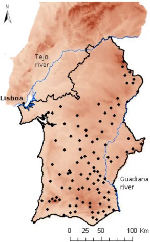
Furthermore, for each station, annual precipitation series were computed and studied for homogeneity through the application of six statistical tests, by means of the hybrid approach proposed by Wijngaard et al. ([15]). In addition, 62% of the long-term series were also checked through relative approaches (testing procedures that use records from reference stations), comprising the application of five homogeneity tests which are capable of locating the year where a break is likely ([2]; [3]). One station’s data was then rejected because multiple break-points were identified and the homogeneous periods were too short and unreliable. Hence, the data used in this study are a set of 105 station records with daily pre-cipitation observations within the period 1940–1999 (Figure 1). Only the longest homogeneous period was used to build the extreme precipitation indices whenever at least one of the relative tests identified a break year.

Figure 1: Study domain and stations’ locations with selected daily precipitation series.

The extreme precipitation indices are sensitive to the number of missing days, thus the selected stations satisfy the following criterion. The daily records are as complete as possible, with less than 16% of data missing in each year. Hence, for each station, the indices for a specific year were set to missing if there were more than 16% of the days missing for that year ([8]).

3. EXTREME PRECIPITATION INDICES

Numerous extreme precipitation indices are described and analyzed in the literature. Some indices involve arbitrary fixed thresholds, such as the number of days per year with daily precipitation exceeding 10mm or 20mm (e.g. [11]; [12]). Other indices are based on statistical quantities such as percentiles, which are more appropriate for regions that contain a broad range of climates ([7]; [11]). Indices based on the count of days crossing certain fixed thresholds are beneficial for impact studies as they can be related with extreme events that affect human society and the natural environment ([11]). Since numerous extreme rainfall in-dices described in the literature are largely inter-correlated, we selected one index representing dry conditions (RL10) and two for wet conditions (R30 and R5D).

The index RL10 is defined as the number of days per year with precipitation amount below 10mm, thus measures the frequency of dry events. The index R30 measures the frequency of extremely heavy precipitation events and is defined as the number of days per year with precipitation amount above or equal to 30mm. The index R5D is defined as the highest consecutive 5-day precipitation total in each year and provides a measure (in mm) of the magnitude of strong precipitation events. In the present study only annually specified indices are considered.

4. METHODOLOGY FOR ASSESSING TRENDS AND

SPACE-TIME PATTERNS IN PRECIPITATION EXTREMES

The extreme precipitation indices were calculated for each station and were then averaged over all the stations to obtain the regional-average of each extreme index per year. The average number of stations series used by year to build the regional-average series is equal to 47. The slopes of the trends in the in-dices of precipitation extremes were calculated by least squares linear fitting and trends’ significance determined using Student’s t-tests. The regression coefficient b (slope) multiplied by 10 gives the change per decade ([11]).

The spatial interpolation of precipitation has been the focus of much re-search (e.g. [14]; [6]; [4]). However, the number of studies analysing space-time patterns of extreme precipitation indices is very limited, as the large majority of the studies focus on the temporal linear trends in the indices. An exception is the work of Hundecha and B´ardossy ([10]) in which the station values of the daily pre-cipitation were interpolated on a 5km×5km grid through external drift kriging, using a digital elevation model as secondary information and, afterwards, several extreme precipitation indices were calculated on grids of 5, 10, 25 and 50 km.

Geostatistical estimators, known as kriging (family of generalized least-squares regression algorithms), provide statistically unbiased estimates of surface values from a set of observations at recorded locations, using the estimated spatial and temporal covariance model of the observed data. Stationarity assumptions on kriging are traditionally accounted for by using local search neighbourhoods so that the dependence on stationarity becomes local ([5]). The most commonly applied forms of kriging use a variogram — inverse function of the spatial (and temporal) covariance. This is a key function of geostatistics and represents the variability of the spatial and temporal patterns of physical phenomena. Usually, a mathematical variogram model is fitted to the empirical semi-variogram values (experimental semi-variogram) calculated for given angular and distance classes. The most common models are the linear, spherical, exponential and Gaussian models ([5]). These models are known as transitive variograms, because the spatial correlation structure varies with the distance h.

The parameters of the variogram model (sill, range and nugget) are then used to assign optimal weights for spatial prediction using kriging. The nugget is determined when h approaches 0. The nugget effect results from high vari-ability at short distances that can be caused by lack of samples, or sampling inaccuracy. The range is one of the most important parameters as it is related with the spatial (or space-time) extent of continuity of the phenomenon. For the case of a spherical model, the range of the variogram is the distance h beyond which the variance no longer shows spatial dependence. At h, the sill value is reached. Observations separated by a distance larger than the range are spatially independent observations.

In this study, the extreme precipitation indices were calculated for each station using data within the baseline period 1940–1999. Afterwards, the space-time patterns of the indices were assessed through ordinary kriging on a 800m× 800m grid, for each year, using a different space-time variogram model for each decade. The way in which the variogram models are chosen and their parameters are estimated is controversial ([5]). In this study we chose exponential models that capture the major spatial features of each attribute under study by subjectively fitting the models to the experimental semi-variogram values taking into account physical knowledge of the area and phenomenon.

It is recognized that topography and other geographical factors are respon-sible for considerable spatial heterogeneity of the precipitation distribution at the sub-regional scale. Precipitation generally increases with elevation because of the orographic effect of mountainous terrain. Ordinary kringing was preferred over other methods incorporating secondary information (e.g., altitude or distance to the coastline) such as cokriging, because of the poor linear relationships (assessed through Pearson’s correlation coefficients) between the three indices and variables such as the elevation and the geographical coordinates of the stations’ locations.

5. RESULTS AND DISCUSSION

5.1. Time trend analysis

The frequency of dry events, measured by the regional average of RL10 within the period 1940–99, is increasing (the change per decade is equal to 0.582 days), but the trend is not statistically significant (the p-value of the t-test is equal to 0.214). The regional average of R30 shows a decrease in the frequency of extremely heavy precipitation events (the change per decade is equal to −0.009 days) but it is not statistically significant (the p-value of the t-test is equal to 0.937). The magnitude of strong precipitation events, measured by the regional average of R5D, is also decreasing (the change per decade is equal to −0.132 mm), but the trend is not statistically significant (the t-test p-value is equal to 0.939).

The variability of the regional-average series of RL10, R30 and R5D does not show significant trends either (Figure 2, left graphics).

5.2. Space-time continuity analysis

The variogram is an inverse measure of the correlation for a given vec-tor distance h. Variograms, which are inverse functions of covariances, describe how the spatial continuity changes as a function of the distance and direction (where anisotropy is considered) between any pair of points in space and time. Variogram’s values increase with increasing distance of separation until they reach a maximum, named sill, at a distance known as the range. Here, the variogram models are a function of these two parameters only, the range (denoted by a) and the sill (denoted by c).

Figure 2: Left graphs: least squares linear fitting (red line) and weighted local polynomial fitting (LOWESS smoothing introduced by [1]) with a time span of 10 years (grey line) for each regional-average series. Right graphs: least squares linear fitting of the regional standard-deviation of RL10, R30 and R5D.

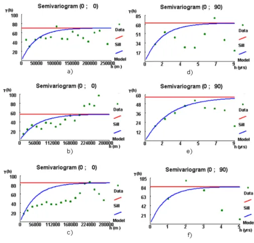
The space-time analysis was done on periods of 10 years: 1940–49, 1945–54, 1950–59, 1954–65, 1960–69, 1965–74, 1970–79, 1975–84, 1980–89, 1985–94, 1990–99. Experimental space-time semi-variograms were calculated for the eleven decades for each extreme precipitation index and exponential models fitted (the spatial component was modelled as isotropic). For sake of simplicity only the variograms of RL10 for 3 decades are shown in Figure 3. The parameters fitted for each var-iogram are summarized in Table 1, showing that there are no relevant tendencies in what concerns the temporal component of the semi-variograms, which is con-sistent with what was previously discussed about the series time trends. However, the ranges of the exponential models fitted to the experimental semi-variograms, which express the extent of spatial continuity of the phenomena, are generally increasing along the decades for all indices. This means that extreme events tend to be more spatially homogeneous along time in this region.

Figure 3: Space-time variograms of RL10 and exponential models fitted. Graphs a), b), c) show the spatial component, and graphs d), e), f) show the temporal component for the decades 1945–54, 1975–85 and 1990–99, respectively.

Table 1: Parameters of the space-time variograms for each precipitation index by decade.

Index Decades Spatial range a_(m) Temporal range a_(years) Sill c

1945–54 120 000 5 70.406 RL10 1975–85 160 000 7.5 56.461 1990–99 275 000 4 71.366 1945–54 60 000 4 11.598 R30 1975–85 100 000 4.5 7.675 1990–99 150 000 4.5 8.984 1945–54 120 000 2.5 2885.47 R5D 1975–85 120 000 3.5 1704.018 1990–99 160 000 1.4 2803.646

5.3. Space-time inference

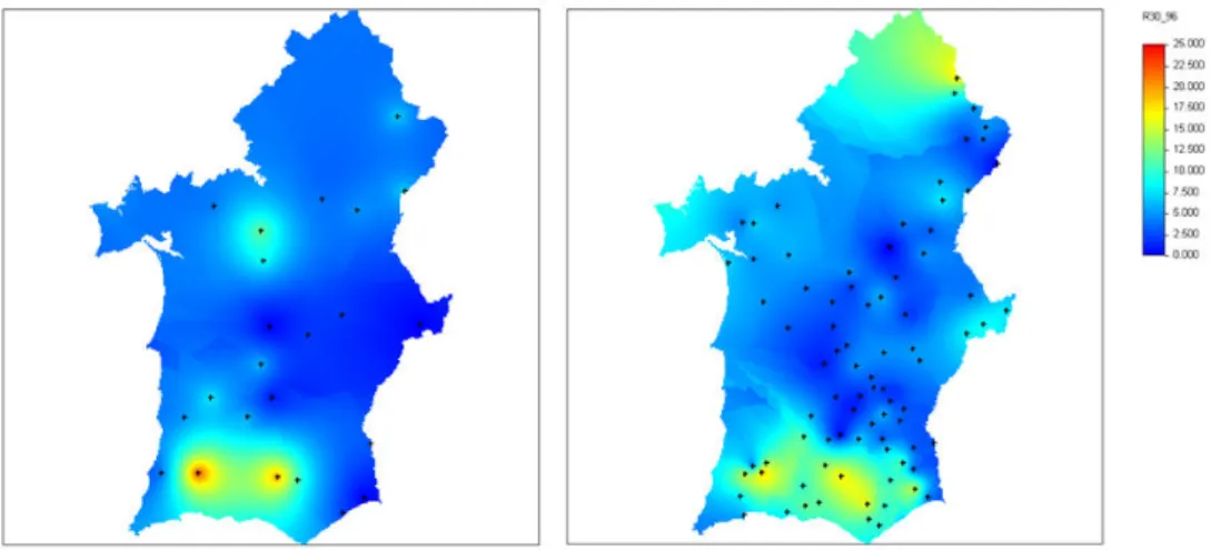
Ordinary kriging was used to estimate in space and time the extreme pre-cipitation indices, producing one map for each index per year. One map from the decade 1945–54 and another one from the decade 1990–99 of each extreme pre-cipitation index are shown in the following figures. The estimated maps of RL10 represent the driest years of those decades, namely 1954 and 1992 (Figure 4). While the estimated maps of R30 represent the wetter years of those decades, namely 1947 and 1996 (Figure 5). The estimated maps of R5D refer to the years with more accumulated precipitation in five consecutive days, namely 1949 and 1997 (Figure 6).

Figure 4: Spatial distribution of the RL10 index for 1954 (left figure) and 1992 (right figure).

Figure 5: Spatial distribution of the R30 index for 1947 (left figure) and 1996 (right figure).

Figure 6: Spatial distribution of the R5D index for 1949 (left figure) and 1997 (right figure).

According with the experimental space-time variograms in the previous sec-tion, the spatial distributions of the three precipitation indexes show an increase of the spatial continuity along time as expected.

6. FINAL REMARKS

The results show no statistically significant trends in the regional-average series within the period 1940–99, although the signs of the slopes are as expected ([11]; ECA project, http://eca.knmi.nl, retrieved April 2007): for the index representing dry conditions the slope is positive and both indices representing wet conditions show negative slopes. However, there is no significant change in the temporal variability of the three regional extreme indices.

All extreme precipitation indices analysed show increased spatial continuity along time.

The results of this application open perspectives for new approaches of the analysis of extreme climate events, particularly in the context of impact studies related with the desertification phenomenon.

REFERENCES

[1] Cleveland, W.S. (1979). Robust locally weighted regression and smoothing scatterplots, Journal of the American Statistical Association, 74, 829–836.

[2] Costa, A.C. and Soares, A. (2006). Identification of inhomogeneities in pre-cipitation time series using SUR models and the Ellipse test. In “Proceedings of Accuracy 2006 — 7th

International Symposium on Spatial Accuracy Assessment in Natural Resources and Environmental Sciences” (M. Caetano and M. Painho, Eds.), Instituto Geogrfico Portuguˆes, 419–428.

[3] Costa, A.C.; Negreiros, J. and Soares, A. (2008). Identification of inho-mogeneities in precipitation time series using stochastic simulation. In “geoENV VI – Geostatistics for Environmental Applications” (A. Soares, M.J. Pereira and R. Dimitrakopoulos, Eds.), Springer, 271–278.

[4] Daly, C.(2006). Guidelines for assessing the suitability of spatial climate data sets, International Journal of Climatology, 26(6), 707–721.

[5] Goovaerts, P.(1997). Geostatistics for Natural Resources Evaluation, Oxford University Press.

[6] Goovaerts, P. (2000). Geostatistical approaches for incorporating elevation into the spatial interpolation of rainfall, Journal of Hydrology, 228, 113–129. [7] Haylock, M. and Nicholls, N. (2000). Trends in extreme rainfall indices for

an updated high quality data set for Australia, 1910–1998, International Journal of Climatology, 20(13), 1533–1541.

[8] Haylock, M.and Goodess, C.M. (2004). Interannual variability of European extreme winter rainfall and links with mean large-scale circulation, International Journal of Climatology, 24(6), 759–776.

[9] Hidalgo, J.C.G.; De Lu´ıs, M.; Ravent´os, J. and S´anchez, J.R. (2003). Daily rainfall trend in the Valencia region of Spain, Theoretical and Applied Cli-matology, 75, 117–130.

[10] Hundecha, Y. and B´ardossy, A. (2005). Trends in daily precipitation and temperature extremes across western Germany in the second half of the 20th

century, International Journal of Climatology, 25(9), 1189–1202.

[11] Klein Tank, A.M.G. and K¨onnen, G.P. (2003). Trends in indices of daily temperature and precipitation extremes in Europe, 1946–99, Journal of Climate, 16(22), 3665–3680.

[12] Kostopoulou, E.and Jones, P.D. (2005). Assessment of climate extremes in the Eastern Mediterranean, Meteorology and Atmospheric Physics, 89, 69–85. [13] L´azaro, R.; Rodrigo, F.S.; Guti´errez, L.; Domingo, F. and

Puigde-f´abregas, J. (2001). Analysis of a 30-year rainfall record (1967–1997) in semi-arid SE Spain for implications on vegetation, Journal of Arid Environments, 48(3), 373–395.

[14] Prudhomme, C.(1999). Mapping a statistic of extreme rainfall in a mountainous region, Physics and Chemistry of the Earth, 24B, 79–84.

[15] Wijngaard, J.B.; Klein Tank, A.M.G. and K¨onnen, G.P.(2003). Homo-geneity of 20th

century European daily temperature and precipitation series, International Journal of Climatology, 23(6), 679–692.