www.atmos-chem-phys.net/9/2075/2009/ © Author(s) 2009. This work is distributed under the Creative Commons Attribution 3.0 License.
Chemistry
and Physics
Spatial heterogeneity of satellite derived land surface parameters
and energy flux densities for LITFASS-area
A. Tittebrand1,*and F. H. Berger2
1Institute for Hydrology and Meteorology, Dresden, Germany
2Deutscher Wetterdienst, Meteorologisches Observatorium Lindenberg, Germany *now at: Institute for Oceanography, Hamburg, Germany
Received: 6 May 2008 – Published in Atmos. Chem. Phys. Discuss.: 26 August 2008 Revised: 20 January 2009 – Accepted: 10 March 2009 – Published: 23 March 2009
Abstract. Based on satellite data in different temporal and spatial resolution, the current use of frequency distribution functions (PDF) for surface parameters and energy fluxes is one of the most promising ways to describe subgrid hetero-geneity of a landscape. Objective of this study is to find typi-cal distribution patterns of parameters (albedo, NDVI) for the determination of the actual latent heat flux (L.E) determined from highly resolved satellite data within pixel on coarser scale.
Landsat ETM+, Terra MODIS and NOAA-AVHRR sur-face temperature and spectral reflectance were used to infer further surface parameters and radiant- and energy flux den-sities for LITFASS-area, a 20×20 km2 heterogeneous area in Eastern Germany, mainly characterised by the land use types forest, crop, grass and water. Based on the Penman-Monteith-approachL.E, as key quantity of the hydrological cycle, is determined for each sensor in the accordant spa-tial resolution with an improved parametrisation. However, using three sensors, significant discrepancies between the in-ferred parameters can cause flux distinctions resultant from differences of the sensor filter response functions or atmo-spheric correction methods. The approximation of MODIS-and AVHRR- derived surface parameters to the reference pa-rameters of ETM (via regression lines and histogram stretch-ing, respectively), further the use of accurate land use clas-sifications (CORINE and a new Landsat-classification), and a consistent parametrisation for the three sensors were real-ized to obtain a uniform base for investigations of the spatial variability.
The analyses for 4 scenes in 2002 and 2003 showed that for forest clear distribution-patterns for NDVI and albedo
Correspondence to:A. Tittebrand ([email protected])
are found. Grass and crop distributions show higher vari-ability and differ significantly to each other in NDVI but only marginal in albedo. Regarding NDVI-distribution func-tions NDVI was found to be the key variable for L.E-determination.
1 Introduction
The land surface interface is a key component of the cli-mate system since it provides the coupling between the at-mosphere and the land biosphere and hydrology (Giorgi, 1996). Up to the present remote sensing is the only observ-ing method for mappobserv-ing land surface characteristics or en-ergy fluxes globally (Liang et al., 2002) with their known uncertainties.
The land surface variables and vegetation variables, such as surface temperature, surface reflectance, Normalised Dif-ference Vegetation Index (NDVI), Leaf Area Index (LAI) and Soil Adjusted Vegetation Index (SAVI) can be derived di-rectly from satellite observations (e.g. Wan and Dozier, 1989; Becker and Li, 1990; Li and Becker, 1993; Ma et al., 2006). The regional radiant and energy flux densities can be inferred only indirectly with the aid of these land surface variables and further vegetation parameters (Pinker, 1990).
The theoretical framework of a satellite based determi-nation of radiant and energy flux densities with focus to the latent heat flux (L.E) based on Penman-Monteith for LITFASS-area (Lindenberg Inhomogeneous Terrain: fluxes between the Atmosphere and the Surface – a long term Study) was given in previous studies (Berger, 2001; Titte-brand et al., 2005) and is presented here with an improved parametrisation for Landsat 7 ETM+ (Enhanced Thematic Mapper) and NOAA 16-AVHRR 3 (Advanced Very High
Resolution Radiometer) data and adapted for Terra MODIS (Moderate Resolution Imaging Spectroradiometer) data.
Parameter and flux distinctions between the sensors result from differences of the sensor filter response functions, cor-rection methods of the atmospheric effect (van Leeuwen et al., 1999; Teillet et al., 1997) or they are based on different or outdated land use classifications (e.g. USGS land cover). Thus, it was necessary to realise comparable land surface pa-rameters to allow a consistent parametrisation scheme for the three sensors. An adaptation method for MODIS (albedo, NDVI and surface temperature) and AVHRR (NDVI) was carried out using the accordant ETM parameters as refer-ence data. An improved and consistent parametrisation for the three sensors led to satisfying findings confirmed by new validation results. The second source of unexplained vari-ability of the resultant fluxes arises from the land use classi-fications. Thus, after comparison to an in-situ land use clas-sification (Beyrich et al., 2004; Beyrich and Mengelkamp, 2006) for LITFASS-area, the Coordinated Information on the Environment classification (CORINE) and a new Landsat-classification (Prechtel, 2005) were used for the study, accor-dant to their spatial resolution for AVHRR (1 km), MODIS (1 km) and ETM (30 m), respectively.
However, the monitoring of vegetation requires data of high temporal resolution which are up to now only pro-vided by sensors with moderate spatial resolution. Their spatial resolution ranges from a few hundred meters (En-visat MERIS, Terra MODIS) up to one kilometer (NOAA AVHRR). While using such moderate resolution data, the heterogeneity of the observed surface could get lost mainly because the landscape is a mosaic of objects such as agricul-tural fields or vegetation patches that are often smaller than the pixel size at a moderate resolution. So the spatial hetero-geneity on an intra-pixel scale will be lost (Garrigues et al., 2006). Thus, high spatially resolved data (e.g. Landsat ETM) are fine enough to describe sub-grid heterogeneity, but at the expense of a coarser repeat cycle of the satellite.
Numerous studies describe different ways of consider-ing sub-grid scale land-surface heterogeneities especially in atmospheric models (Arain et al., 1996; Avissar, 1992; Chebouni et al., 1995; Koster and Suarez, 1992a, b; Lhomme et al., 1994; Li and Avissar, 1994; Noilhan et al., 1997; Sellers et al., 1997; Shuttleworth et al., 1997). Basically, three methods have been developed: The Usage of effective parameters (Arain et al., 1996; Lhomme, 1992; Claussen, 1995a) have been proposed as a means for applying equa-tions developed for homogeneous or point-scale processes, to processes occurring at larger spatial scales over heteroge-neous surfaces. One method for deriving expressions for the effective parameters is to express the energy balance equa-tion separately in terms of effective and component surface parameters, and then to match the expression term by term using some initial assumption about which fluxes will be “conserved” in going from the small to the large scale (Njoku et al., 1996). The “tile” approach (Li and Avissar, 1994)
describes the heterogeneity inside a model grid cell in terms of a number of homogeneous “tiles” representing the domi-nant vegetation and soil types. The grid fluxes are the aver-ages of the tile fluxes weighted by their fractional area. For the “mosaic” approach (Koster and Suarez, 1992a; M¨olders and Raabe, 1996) the model grid cell is subdivided into a reg-ular smaller high-resolution grid. While the coarse grid for the host model is preserved, the SVAT scheme is used for the smaller grid. The averages of the sub-grid fluxes represent the fluxes on the coarse grid. In a SVAT scheme a number of parameters are used to describe the soil and vegetation char-acteristics inside the grid cell. These parameters are usually selected in correspondence to the most common vegetation and soil types within the grid square.
The usage of frequency distributions or generalized prob-ability density functions (PDF) offers another possibility to describe the variability of land-surface characteristics, at a resolvable scale of interest (Li and Avissar, 1994). This statistical-dynamical approach (Entekhabi and Eagle-son, 1989; Avissar, 1992; Bonan et al., 1993; Giorgi 1996a, b) is needed because of the nonlinear relationship between most land-surface characteristics and the land surface heat fluxes. Therefore PDF could be used to describe spatial vari-ability of a specific surface parameter for a satellite pixel or a model grid with coarser spatial resolution that is described by a higher resolved data set (MAGIM, 2006). The PDF can replace the use of effective parameters or other specific aver-aging strategies. Furthermore it considers the extreme values as well as the mode which can be completely different from the simple mean. This method was used by Giorgi (1996a, b) with the PDF of soil moisture and surface temperature to de-scribe the representation of surface heterogeneity to be used in climate models. Li and Avissar (1994) demonstrated that the results of determined fluxes depend on the shape of the spatial distribution of the land surface parameters, used for the calculation. Typically, the more skewed the distribution within the range of values the larger the error (for nonlinear relationships) of the flux calculated using the mean instead of the distribution. Investigations in our study focus espe-cially on the determination of latent heat and the distribution patterns of the needed parameters (e.g. albedo, NDVI).
The spatial heterogeneity of parameters and energy fluxes in their given spatial resolution was first investigated us-ing statistic quantities. For comparison of the results for the different satellite sensors a common spatial resolution is needed, thus two different averaging methods are tested and compared (arithmetic mean and the dominant land use method). The heterogeneity of the parameter and fluxes is then described by the characterisation of their frequency dis-tributions (a) for the entire target area, (b) considered for sev-eral land use types and (c) on pixel base. Based on this work, typical patterns for the use of the PDF-method for the de-termination ofL.E (using the Penman-Monteith approach) could be provided determined from the highly resolved ETM data within pixel on coarser scale (MODIS, AVHRR).
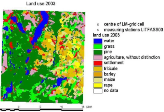
Fig. 1.Land use classification of LITFASS-area from in-situ refer-ence data 2003.
2 Target area and data
2.1 Target area
The study focuses on a 20 km×20 km area around the Richard Aßmann Observatory (MOL-RAO) of the German Meteorological Service (Deutscher Wetterdienst, DWD) sit-uated in North Eastern Germany 50 km Southeast of Berlin. The land use in this area is dominated by forest and agricul-tural fields with approximately 45% each, lake coverage of 7% and villages cover nearly 4%. The forest is dominated in the Western part of the area while agriculture is mainly sit-uated in the Eastern part (Fig. 1). The target area is formed by inland glaciers, exhibiting a flat surface with differences of only 80–100 m over distances of about 10–15 km with a number of small and medium-sized lakes (Mengelkamp et al., 2006)
2.2 Satellite data and time
The investigation is carried out with Landsat-7 ETM+, Terra MODIS and NOAA 16 AVHRR 3 data. Landsat-7 ETM+ data, provided as Level 1B data, offer a spatial resolution of 30 m with a 16 day repeat cycle. The determination of brightness temperature and spectral reflectance on top of at-mosphere (TOA) was applied after the Landsat User Hand-book (2004).
From MODIS surface temperature and reflectance prod-ucts from the Earth Observing System Data Gateway were used (EOS, 2007) for the determination of NDVI as well as for further parameters for the calculation of the energy fluxes. The reflectance product MOD09GHK was estimated for each band to produce a measurement equivalent to a ground-level measurement with no atmospheric scattering or absorption. The correction scheme identifies atmospheric gases, aerosols and thin cirrus clouds. These MOD09GHK data are provided as a grid-level-2G, 500 m product in the sinusoidal projec-tion. MODA11 temperature data were used, also given as a
gridded product with a 1 km spatial resolution and corrected for the atmospheric effect.
In former studies of the institute NOAA 16-AVHRR 3 data were processed with the modularic scheme SESAT (Strahlungs- und Energiefl¨usse aus Satellitendaten, Berger, 2001; Tittebrand et al., 2005). For a comparable determi-nation of the energy fluxes according to ETM and MODIS in this work only surface temperature (after Mc Clain, 1985; split window method), spectral reflectance and TOA-NDVI (Top of Atmosphere) of SESAT were used, given with a 1 km spatial resolution. For this case study four cloud free scenes in spring and summer 2002 and 2003 were used: 9 May 2002, 28 July 2002, 20 August 2002 and 17 April 2003.
For evaluation purposes a field experiment (Beyrich and Mengelkamp, 2006) was planned and realised in May until June 2003. At that time two cloud free Landsat-overpasses were recorded. Unfortunately on 31 May 2003 problems with Landsat’s scan line corrector occured (Landsat, 2003) thus these scenes were not available for the analysis. Only the cloud free scene a couple of weeks earlier (17 April 2003) could be used. Spring and summer 2003 were dry in contrast to the summer 2002, especially in August 2002, where the scene was taken only a few days after the flash-flood in East-ern Germany. So it was of interest to determine the latent heat flux under various soil moisture and atmospheric con-ditions. For comparison half-hourly in-situ measurements of the routine observations in Lindenberg (Beyrich et al., 2004) were used but with absence of data of the turbulent fluxes except for the April scene in 2003.
2.3 Land use classifications
To use the best appropriate land use classification two land use classifications with fixed resolutions were testet:
– 1 km: CORINE (Coordinated Information on the Envi-ronment) is a consistent, comparable use and land-cover data base for the European environmental policy. To meet the requirements a satellite based (Landsat-7 ETM+) pan-European initial data acquisition of land use/cover types has been carried out.
– 25 m: Landsat-classification 2002 was developed by the Institute of Cartography of the Technical University of Dresden based on two Landsat-7 ETM+ scenes of Sax-ony in Germany to support the satellite retrieval algo-rithm for parameter and flux determination.
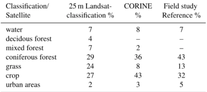
A comparison of the percentage representation of the main land uses for LITFASS area is shown in Table 1 for the land use classifications compared to field data. Further informa-tion about these classificainforma-tions is given in the appendix. For the comparison of land use classifications consistent classes had to be found. Therefore classes containing for example different field fruits were summarized to one class: crop. Nevertheless there are bigger differences between not only
Table 1. Comparison of the land-use classifications CORINE and Landsat-classification that are used for the satellite data for LITFASS-area with the reference classification (Beyrich et al., 2004; Beyrich and Mengelkamp, 2006) based on a field study in 2003.
Classification/ 25 m Landsat- CORINE Field study Satellite classification % % Reference %
water 7 8 7
decidous forest 4 – –
mixed forest 7 2 –
coniferous forest 29 36 43
grass 24 8 13
crop 27 43 32
urban areas 2 3 5
the percental representation of each class but also for the classification. A good agreement can be found for the wa-ter classes compared to the reference classification. Actually in LITFASS-area there is no deciduous forest (Fig. 1). Both classifications match this well and give coniferous forests as dominant land use type for high vegetation. Nevertheless, regarding Table 1, coniferous forest is underestimated for CORINE and Landsat-classification with differences of 14% and 7%, respectively compared to the reference. Most uncer-tainties can be outlined for crop and grass, probably because of their similar spectral behaviour. For both land use types their differences are higher to each other than to the refer-ence classification which possesses values in between. As mentioned above and outlined in Keil et al. (2005) CORINE tends to overestimate agricultural areas. Compared to the ref-erence classification of LITFASS-area (Beyrich et al., 2004; Beyrich and Mengelkamp, 2006) CORINE and the Landsat-classification showed nearly comparable results. Thus they are applied here to the satellite data, according to their spa-tial resolution: the CORINE classification for MODIS and AVHRR analyses and the Landsat-classification for ETM data. For flux determination the classifications were reduced to four classes: forest, grass, crop and water. Remaining classes were assigned to one of the four classes, as e.g. urban areas to the forest class because of the comparable roughness length (Beyrich et al., 2004).
3 Satellite derived fluxes and adaptation due to sensor differences
3.1 Satellite based parameters
To solve the Penman-Monteith equation the only satellite based quantities were surface spectral reflectance (and hence broadband albedo), NDVI and surface temperature.
The ETM-broadband albedo was inferred using chan-nels 1, 3, 4, 5 and 7 after Liang et al. (2002) after the correction of atmospheric effects using 6 S (Vermote et al., 1995). Surface temperature was determined after Sobrino et al. (2004) using a single windows channel method for chan-nel 6. The NDVI=(ρNIR-ρVIS)/(ρNIR+ρVIS) for ETM is based on reflectance in channel 3 and in channel 4.
MODIS-broadband albedo was consistently computed af-ter Liang et al. (2002) using channels 1 to 5 and 7. NDVI can be derived combining channel 1 and 2. For determination of the MODIS-fluxes the spectral reflectance data were aver-aged to the 1 km (interpolated 800 m) resolution allowing the combination of reflectance and temperature (both products provided), NDVI and surface temperature derived as men-tioned above are the base for the determination of further pa-rameters (e.g. LAI) and their resulting energy fluxes.
For AVHRR albedo and TOA-NDVI and surface temper-ature were used from the SESAT scheme (Berger, 2001) as base for energy fluxes.
3.2 Determination of surface fluxes
As described in Tittebrand et al. (2005) the Penman-Monteith method was used to infer the actual latent heat fluxes on satellite-pixel base for the LITFASS-area assuming constant boundary layer conditions. Therefore the difference of net radiation (Rn) and soil heat flux at the surface (G), to be termed available energy, and a couple of further parameters (LAI, roughness length, wind speed, relative humidity and others) are needed. The approach is given as follows: L.EPM=
s
s+γ1+rc
ra
(Rn−G)+ (1)
1 s+γ1+rc
ra
ρcp
ra
(es(T2 m)−e(T2 m))
here Rn-Gis the available energy from net radiation Rn and surface soil heat fluxG, sis the slope of the saturation vapor versus temperature curve,ρthe air density in kg m−3,cpthe specific heat of air at constant pressure,y the psychrometric constant, andes(T2 m)−e(T2 m)the saturation deficit (es
ac-cording to Magnus-Equation, Sonntag, 1982). The temper-ature in 2 m height is determined fromTsur−T2 m=G/AG
after De Rooy and Holtslag (1999) withAG=9 Wm−2K−1.
The aerodynamic resistancerais derived from the
logarith-mic wind profile:
ra=
0.74 k2u
2 m
ln(z−d) z0
2
(2) with the Karman constant k=0.4, z−d the measurement height above the zero plane displacement,z0the roughness length andu2 mthe wind speed at 2 m. Because these quan-tities are not available for each single pixel the parameteri-sation ofrais realised with land use dependent values forz0
and vegetation height according to Hagemann (2002). Wind speed and relative humidity were included from in-situ tower measurements of the Observatory Lindenberg (MOL-RAO) for the respective time of overpass. In case of no data the boundary layer conditions are assumed to be constant (rela-tive humidity RH=55%, visibility=23 km, wind speed=3 m/s) and they are used for the entire area. The canopy resistancerc
is given by Allen (1986) and Allen et al. (1998): rc=
rs
LAIactive (3)
with LAIactive the fraction of leaf area which actively contributes to vapour transport and here defined as LAIactive=0.5 LAI.
The stomatal resistance rs is a plant specific parameter
depending to some extent on light intensity, temperature, leaf-air vapor pressure difference and ambient CO2 concen-tration. Canopy resistance describes the resistance of wa-ter vapor transport through the entire transpiring vegetation canopy. For lower vegetation without water stress Allen et al. (1998) give a value of about 100 s m−1. Minimum r
s
of forest stands show quite a range. Kelliher et al. (1995) give as maximum leaf stomatal conductance 5.7±2.4 mms−1 (equivalent torsmin=123. . . 303 s m−1)for conifer forest and
4.6±1.7 mms−1 (equivalent to rsmin=158. . . 345 s m−1) for
deciduous forest. Breuer et al. (2003) show even broader spans withrsminwell beyond 700 s m−1for species of both types. In this study for forest 400 s m−1, for low vegetation 100 s m−1 and as an approximation for mixed lower/forest vegetation 250 s m−1were used.
In the study the LAI is computed according to the land use information of the LITFASS-area. To determine the LAI, for certain land use classes empirical relations from field studies are assigned based on the given land use as mentioned above. Grass and the different forms of crop are summarised in one group with lower vegetation. Therefore the approach of Bach et al. (2000) is used with:
LAI=(1.86·NDVI)6.06 (4)
for coniferous forest LAI is given by Bach et al. (2000) with:
LAI=(1.6·NDVI)3 (5)
The sensitivity of the used parameters and their influence on the determination ofL.Eis described in detail in Tittebrand et al. (2005).
Providing all needed parameters for the Penman-Monteith approach the radiation and energy fluxes can be inferred: the net radiation at surface is computed as the sum of the individ-ual short- and longwave flux densities. Partly these compo-nents are achieved using an inverse remote sensing approach, so called look-up tables (LUT). Insolation at surfaceRgand
incoming longwave radiation emitted by the atmosphere are calculated with the radiation transfer code Streamer (Key, 1999) over the entire short- and longwave spectra for the con-ditions of the specific date. Reflected shortwave radiation is
calculated fromRgand the surface reflectance of each pixel.
Outgoing longwave radiation is computed from surface tem-perature using Stefan-Boltzmann law.
Soil heat fluxGfor lower vegetation (grass and crop) is calculated using the approach by Gao (1998):
G=0.539SR−0.53e−K/cosθ0 ·Rn (6) With the simple ratio SR=(1-NDVI)/(1+NDVI), the con-stantKand the sun zenith angle. For forest stands the canopy storage is added to the soil heat flux, based on field studies in Tharandt (near Dresden) for spruce measurements and here used for satellite derived fluxes:
Gg=ag+bg·Rn (7)
Gj =aj +bj·Rn (8)
G=Gg+Gj (9)
withGg the soil heat flux,Gj the canopy heat flux andG the resultant entire surface soil heat flux for forest. The co-efficients ag,bg, aj andbj resultant on linear regressions and are time dependent and used due to the time of satellite overpass (Berger, 2001).
To complete the energy balance equation (Rn=L.E+H+G), the sensible heat flux H is calcu-lated and not inferred as residuum with the variables as mentioned above:
H =ρcp
TS−T2 m
ra
(10) 3.3 Sensor-adaptation
Differing in range, shape and different influences by water vapour, the differences in the filter response functions of the three sensors have a strong influence on the determination of spectral reflectance and can result in a sensor-dependent NDVI (van Leeuwen et al., 1999; Teillet et al., 1997; Batra et al., 2006) and hence in differing results in the energy fluxes. In this work the ETM results are treated as reference con-cerning the best validation results of the three satellites in comparison to in-situ measurements of grass in Lindenberg for all four scenes. Realising comparable fluxes besides the mentioned differences in sensor features and filter response functions, the AVHRR and MODIS fluxes should be com-puted using the same parameters and assumptions as used for the ETM data. Comparing ETM- (arithmetically aver-aged to MODIS-resolution) and MODIS-albedo, NDVI and surface temperature for each pixel, high correlation coeffi-cients for the four investigated scenes 9 May 2002, 17 April 2003, 20 August 2002 and 28 July 2002 could be found: tem-perature (r=0.66, 0.79, 0.78 and 0.75, respectively), albedo (r=0.95, 0.97, 0.90 and 0.93) and NDVI (r=0.79, 0.92, 0.89 and 0.89). That allowed the usage of the regression lines for correction/shifting (approximate to the 1:1 agreement) and therefore to create comparable MODIS-parameters for the
0 5 10 15 20 25 30 35
fr
e
q
u
e
n
c
y
%
0,0 0,2 0,4 0,6 0,8 1,0
NDVI
ETM_NDVI
MODIS_NDVI_uncorr AVHRR_NDVI_uncorr
original resolution
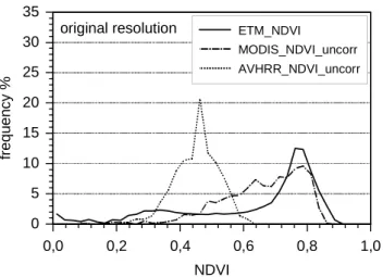
Fig. 2. Differences in NDVI determined with the three sensors in
their given spatial resolution, note that AVHRR-NDVI is uncor-rected for atmospheric effects (TOA), for 20 August 2002.
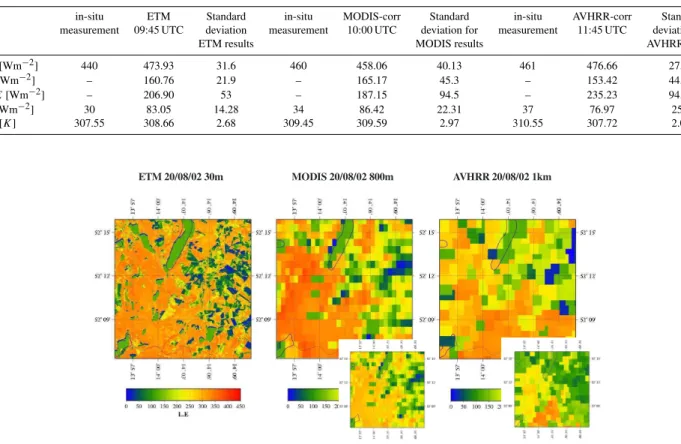
according ETM-parameters. Especially the MODIS surface temperatures showed much lower values before and could be seen as the reason for the deviations e.g. in Rn between ETM and MODIS for all scenes. For AVHRR surface temperature, albedo and TOA-NDVI were used from the SESAT scheme as base for the new calculation of the en-ergy fluxes. Because of the 2 h delay of the AVHRR over-pass (AVHRR measurements are close to the noon maxi-mum in contrast to MODIS measurements at 10:00 UTC) the regression-adaptation-method should not be used for these sensor differences. The data analysis showed that an adap-tation of NDVI – which is significantly lower for AVHRR (Buheaosier et al., 2003; van Leeuwen et al., 2006) than for ETM and MODIS (Fig. 2), is sufficient to infer compara-ble energy fluxes. NDVI adaptation was realised by stretch-ing the NDVI-distribution histograms. Energy and radiant fluxes are then calculated according to the ETM algorithm, because of the comparable NDVI. Surface temperature was in good agreement compared to in situ data and therefore not changed. The resultant L.E fluxes for the three sen-sors are shown in Fig. 3 in their given spatial resolution and for MODIS and AVHRR (smaller plots middle and respec-tively right) in the former computation for 20 August 2002. Comparing the original fluxes to the fluxes with parameter adaptation a significant improvement could be achieved not only for the range ofL.Ebut also for the spatial distribution of the values especially for AVHRR. A confinement accord-ing to water values had to be found usaccord-ing constant values L.E=125 Wm−2because the Penman-Monteith method was not applicable for water bodies. These plots are treated as the base for further analysis concerning spatial heterogene-ity including investigations according to standard deviations, averaging methods and analysis of frequency distributions of fluxes and parameters.
Table 2 shows exemplarily the validation results from the 20 August 2002 compared to the grass-station of Lindenberg for ETM (original), MODIS (corrected) and AVHRR (cor-rected). Due to uncertainties in the geolocation especially of the AVHRR scenes also ambient pixels around the target pixel are extracted and averaged to achieve a relative statistic certainty to encounter the location of ground measurements. The results, given in Table 2 show an excellent agreement for Rn and surface temperature. Indeed ETM-Rn seems to overestimate at about 30 Wm−2 but taking the standard de-viation into account the in-situ measurement lies within the error bars. Soil heat fluxGremains an uncertain and hard to derive quantity with overestimations of all sensors of 40– 50 Wm−2. Values for the turbulent fluxes are missing for this day but taking the other quantities into account – the evapora-tion can be assumed to fit well, especially for these very wet conditions in August 2002, although LITFASS-area is domi-nated by sandy soils with high infiltration.His computed us-ing Eq. (10) and not the remainus-ing quantity of the energy bal-ance. So the system is open, but with only small gaps in the energy balance (ETM: 23.22 Wm−2, MODIS: 19.32 Wm−2 and AVHRR: 11.04 Wm−2).
Validation data from the MOL-RAO for the turbulent fluxesL.EandHare only available for 17 April 2003 and in comparison to the ETM data the satellite derived fluxes are in good agreement for latent heat with 93 Wm−2(in-situ mea-surement) versus 72.25 Wm−2 (standard deviation=20.58) inferred from the satellite data, but forH with 48 Wm−2(in situ) versus 118.96 Wm−2(standard deviation=12.79), with higher deviations. The comparison between in-situ data and MODIS- as well as AVHRR results for the turbulent fluxes shows significant higher deviations than for ETM. To gain comparable energy fluxes of the three sensors they had to be averaged onto the same spatial resolution. Figure 4 shows the LITFASS-mean inferred from ETM and MODIS data that were averaged to a comparable AVHRR-resolution (1.1 km). Two averaging strategies are used: a simple mean (arithmeti-cally, left) and the average based on the dominant land use-method (right). Additionally standard deviation (red bar) is given. The sensor-means differ only marginal compared to each other as well as for the averaging methods in each of the Figures.
Between the two averaging-methods a correlation of r=0.94 could be found for L.E. The distributions of the values (Fig. 5) show obvious differences regarding the shape while the range mainly remains. For both methods the range is narrower compared to the original ETM-L.Edistribution. Nevertheless, while using only the mean value of all pixels which are part of the dominant land use type, the shape better agrees with the reference. However, by the usage of the PDF approach improvements according to the results are promised taking the entire range and shape of the distribution of the pa-rameter for flux determination into account.
Table 2. Validation results for corrected (corr) energy flux densities (net radiation (Rn), sensible heat flux (H), latent heat flux (L.E) and soil heat flux (G)) and surface temperature (T s) for 20 August 2002.
in-situ ETM Standard in-situ MODIS-corr Standard in-situ AVHRR-corr Standard measurement 09:45 UTC deviation measurement 10:00 UTC deviation for measurement 11:45 UTC deviation for
ETM results MODIS results AVHRR results
Rn [Wm−2] 440 473.93 31.6 460 458.06 40.13 461 476.66 27.11
H[Wm−2] – 160.76 21.9 – 165.17 45.3 – 153.42 44.07
L.E[Wm−2] – 206.90 53 – 187.15 94.5 – 235.23 94.17
G[Wm−2] 30 83.05 14.28 34 86.42 22.31 37 76.97 25.5
T s[K] 307.55 308.66 2.68 309.45 309.59 2.97 310.55 307.72 2.04
ETM 20/08/02 30m MODIS 20/08/02 800m AVHRR 20/08/02 1km
Fig. 3.RecalculatedL.Efluxes for 20 August 2002 for MODIS (middle) and AVHRR (right) in their given spatial resolution, based on the
Penman-Monteith approach, using the same parametrisation as for ETM (left). (Small plots show the determined preliminary fluxes before, without adaptation to the ETM-parameters.)
4 Density functions – results and discussion
As briefly shown in the previous chapter the distribution of values can give further information concerning heterogene-ity. LITFASS-mean is nearly the same for some fluxes be-tween the different sensors. But the question is whether it possible to find typical PDF of parameters and fluxes for se-lected land use classes?
We split here the overall frequency distribution into land use classes, resulting in individual PDF of Albedo, NDVI andL.E. focus is given to the question whether it is it neces-sary to differentiate between crop and grass or if it is enough to have one “low vegetation” class. Therefore a land use dependent distribution was realised based on the Landsat-classification for ETM and on CORINE for MODIS and AVHRR. For the analysis the left panel of Fig. 5 was inves-tigated according to the land use types grass, crop and forest with respect to the question: which land use class provides which patterns? Figure 6 shows exemplarily the frequency distribution for albedo and NDVI (as example for satellite derived parameters) and the resultantL.Efor ETM on the 20 August 2002.
First: for albedo (left side of Fig. 6), completely different patterns can be found for forest compared to crop and grass, which show very similar distributions as expected. Highest frequency for forest is around 11–12% according to the dark color of the forest including nearly 100%Pinus Sylvestris. Crop and grass values rise slowly from 10% on, finding the peak around 17–19% (more obvious for crop) and then de-scending again. Second: NDVI (middle) andL.E(right side) show a strong agreement in their distribution-patterns, so the key parameter NDVI can be found clearly in theL.Eresults. For August it can be pointed out that NDVI differs clearly for crop and grass. Indeed there is a comparable frequency maximum at NDVI=0.78 andL.E=320–340 Wm−2but for crop a second peak is found for NDVI=0.3, which is a typ-ical value for old vegetation or a significant soil part, and withL.E=40–60 Wm−2. Depending on the type of crop or time of the harvest this peak is significant or not and can not be found for grasslands. For pine the frequency maximum can be found for 0.8 and 320 Wm−2 for NDVI and L.E, respectively. The classes with smaller NDVI andL.E are less represented and only caused by the understory. Analy-sis (distribution functions and areal plots) of NDVI andL.E
0 100 200 300 400 500 600
fl
u
x
e
s
[W
m
];
T
[K
]
-2
S
ETM MODIS AVHRR
Rn L.E H G Ts
LITFASS-mean, arithm. averaged
0 100 200 300 400 500 600
fl
u
x
e
s
[W
m
];
T
[K
]
-2
S
ETM MODIS AVHRR
Rn L.E H G Ts
LITFASS-mean, dominant. averaged
Fig. 4. Mean and standard deviation (std) of the energy fluxes and surface temperature for LITFASS-area for 20 August 2002, arithmetic
mean (left), dominant land use method (right), both averaged to AVHRR resolution (1.1 km).
Fig. 5.Frequency distribution of ETM-L.Efor 20 August 2002 with original resolution (left), arithmetic mean (middle), dominant land use
method (right), both averaged to MODIS resolution (800 m).
show a direct relationship for all land use types. Thus it can be pointed out the higher the NDVI (and thus the LAI) the higher the L.E inferred with Penman-Monteith. With ex-ception for crop- and grass-albedo which are more or less regularly distributed, the mean (given within the diagrams in Fig. 6) and mode of the distribution functions are unequal especially for NDVI andL.E of grass and crop noticeable by the considerable skew of the functions. Sensitivity stud-ies show that a change in LAI from 1 to 3 (e.g. caused by an NDVI increase from 0.51 to 0.78 (mean and mode re-spectively, here for crop from Fig. 6 middle) and in depen-dence on the used NDVI-LAI relationship, can results in an increase of L.E up to 162 Wm−2 (Berger and Schwiebus, 2004; Tittebrand et al., 2005).
Using different land use classifications for ETM and MODIS/AVHRR data can result in uncertainties according to disagreement of the corresponding classes. Thus a pixel in-vestigation should show whether the entirety of all ETM pix-els within one MODIS-pixel show the same dominant land use compared to the accordant MODIS pixel itself. Ten ran-domized MODIS pixels for each land use class (grass, for-est and crop) are collected for the invfor-estigation including approximately 600 ETM pixels for comparison. If at least 80% of the ETM pixels provide the same land use type as the MODIS pixels, statements according to the representa-tiveness of the distribution-patterns should be allowed. A good agreement can be found for the forest class whereas it
was difficult to differentiate between crop and grass classes that are often interchanged between Landsat-classification (ETM) and CORINE (MODIS). Figure 7a shows the fre-quency distributions of Rn for grass (left), crop (middle) and forest (right) for the 28 July 2002 as an example.
The variability of the Rn distributions representing the same land use is highest for crop followed by grass and forest. While for grass and forest there is one significant peak at about 500 Wm−2and about 600 Wm−2, respectively, for crop different frequency peak positions (dominating at about 440 Wm−2and 550 Wm−2)occur. The range is much broader and the distributions differ from each other. This variability is explicable by the different kinds of crop that are summarised within this group providing different reflectance or vegetation indices due to their appearance.
RegardingL.E in Fig. 7b for all land use types a broad range occur but also with observable peak positions. Compa-rable higher variability of the ETM distributions for grass and crop is found whereas for forest the distributions are closed to each other providing one significant peak for all at about 350 Wm−2).
These analyses are further repeated for early summer (9 May 2002) and late summer (20 August 2002). Summa-rizing, it can be outlined that each land use type provides typical distribution patterns both for the selected parameters of the Penman-Monteith approach and the resultant fluxes. Changes of their peak-positions are according to seasonal
Fig. 6. Frequency distributions of albedo (left column), NDVI (middle column) andL.E(right column) for 20 August 2002 for different land use types (grass, crop, forest).
60
fr
e
q
u
e
n
c
y
[%
]
60
fr
e
q
u
e
n
c
y
[%
]
100
fr
e
q
u
e
n
c
y
[%
]
0 10 20 30 40 50 60
fr
e
q
u
e
n
c
y
[%
]
300 400 500 600 700 800 900
Rn [Wm ]-2
28/07/02 grass
ETM-distributions for 4 MODIS-pixel
0 10 20 30 40 50 60
fr
e
q
u
e
n
c
y
[%
]
300 400 500 600 700 800 900
Rn [Wm ]-2
28/07/02 crop
ETM-distributions for 5 MODIS-pixel
0 20 40 60 80 100
fr
e
q
u
e
n
c
y
[%
]
300 400 500 600 700 800 900
Rn [Wm ]-2
28/07/02 forest
ETM-distributions for 6 MODIS-pixel
Fig. 7a.Frequency distribution of ETM-Rn for 28 July 2002 for grass (left), crop (middle) and forest (right), within the accordant MODIS
pixels.
changes. The typical shapes of the density functions are seen to be stable and therefore useful for PDF-applications. In general PDF for NDVI, Albedo, Rn and further parameter could be used to generate PDF of latent heat. The advan-tage is then the consideration of the natural heterogeneity of the surface by taking the entire range of the distributions of the parameters into account. However theL.E determina-tion is based on many variables and assumpdetermina-tions that can be affected by missing satellite measured parameters.
5 Conclusions and outlook
In this study an investigation of the heterogeneity of land sur-face parameters and energy fluxes for LITFASS-area (Ger-many, 50 km Southeast of Berlin) was carried out.
Therefore some preliminary work had to be done to ensure the comparability of the results including the elimination of sensor differences between ETM, MODIS and AVHRR. This was obtained through adaptation, using regression lines of surface temperature, albedo and NDVI for MODIS and his-togram stretching of the NDVI for AVHRR, with reference to
0 10 20 30 40 50 60 fr e q u e n c y [% ]
0 100 200 300 400 500
L.E [Wm ]-2
28/07/02 grass
ETM-distributions for 4 MODIS-pixel
0 10 20 30 40 50 60 fr e q u e n c y [% ]
0 100 200 300 400 500
L.E [Wm ]-2
28/07/02 crop
ETM-distributions for 5 MODIS-pixel
0 20 40 60 80 100 fr e q u e n c y [% ]
0 100 200 300 400 500
L.E [Wm ]-2
28/07/02 forest
ETM-distributions for 6 MODIS-pixel
Fig. 7b.Frequency distribution of ETM-L.Efor 28 July 2002 for grass (left), crop (middle) and forest (right), within the accordant MODIS
pixels.
ETM. Thus the sameL.E-determination method for all sen-sors could be realised. The results show reasonable agree-ment with in-situ data of the observations in Lindenberg.
Due to the land use based parametrisation for flux de-termination new land use classifications were used: the Landsat-classification (TU-Dresden, 25×25 m2)was applied for ETM data and, CORINE (1×1 m2)was used for MODIS and AVHRR data showing good agreement in comparison to in-situ data for LITFASS-area. Nevertheless, differences re-main, e.g. an overestimation of the crop classes of CORINE or an underestimation of water areas (Keil et al., 2005). The quality criterion for the Landsat-classification was an accu-racy of 5% which had to be reached. Based on the same de-termination method and comparable land use classifications for the different sensors, a variability analysis has been car-ried out.
LITFASS-mean and standard deviations for averaged data (arithmetically and using the dominant land use method) were investigated. It was demonstrated that the LITFASS-mean of the fluxes is nearly comparable irrespective of whether it is arithmetically or dominant averaged. For all fluxes the standard deviation for arithmetically averaged data is lower than for dominant land use averaged data.
The heterogeneity analysis was carried out with respect to frequency distributions for the land use classes grass, crop and forest to find typical patterns of their distribution func-tions and the comparability and variability of ETM parame-ters or flux distributions on MODIS-pixel base.
The analysis with respect to land use classes show differ-ences in the distribution patterns, not only between grass and forest but also between grass and crop. One question of the study was to investigate whether it is possible to summarize both classes to one group e.g. lower vegetation. Thus, for further studies using the PDF e.g. forL.E-determination it is suggested to differentiate between crop and grass because a second peak for crop showing the bare soil conditions in the distributions of NDVI and thusL.Eappears (in three differ-ent seasonal states of summer) that can not be neglected.
Selecting MODIS pixels with known land use classes and analyzing therefore their included ETM-distributions (consisting of approximately 600 pixels each), allowed
conclusions with respect to pixel-heterogeneity, assuming that they represent the same land use type (at least 80%). The distribution variability ofL.Eis shown to be higher than for Rn except for the crop class where an evident difference in the distribution patterns can be found. The best distribution agreement can be outlined for forest. According to spatial variability of L.E former studies also showed that the la-tent heat flux was the most sensitive parameter for that issue (Li and Avissar, 1994). Thus the results indicate that it is very important to consider the spatial variability of NDVI and therefore LAI, stomatal resistance, as well as further im-portant parameters and fluxes (surface temperature, Rn and G) of the Penman-Monteith approach.
Averaging highly resolved satellite data arithmetically or using dominant land use gives only marginal differences, but it is assumed that using PDF and thus the entire range of the surface characteristics, including extremes as well as the mode instead of the mean, should provide more realistic con-ditions for the determination of energy fluxes. Li and Avis-sar (1994) confirmed that the results of determined fluxes depend on the shape of the spatial distribution of the land surface parameters, used for the calculation. Typically, the more skewed the distribution within the range of values the larger their error (for nonlinear relationships between param-eter and flux e.g.: for LAI, inferred nonlinear from NDVI). They found largest differences for lognormal distributed land surface parameters and showed that the shape of the distri-bution is essential for the determination of accurate fluxes. Our preliminary results (MAGIM, 2006) confirm the possi-ble application of the PDF-approach for the determination of latent heat flux with Penman-Monteith using NDVI, albedo, relative humidity and wind speed for grassland and conifer-ous forest. Assumingχ2-distributions with a different range and mode for grass and forest, the method was applicable for these two land use types as a first approximation. The approach can now be improved by the new distribution pat-terns of the parameters for the two land use types and by the enhancement for the often represented land use type “crop” with a clearly different distribution function compared to grass – especially for NDVI as the key variable for the L.E-determination using Penman-Monteith.
Finally, realising theL.E-determination with the PDF ap-proach offers new interpretation of validation results. Un-til now pixel mean and standard deviation were compared to point measurements often resulting in significant differ-ences. Taking the entire PDF of the resultant latent heat flux for comparison into account, the in situ measurement can be different from mean or mode and nevertheless be representa-tive for the pixel.
Appendix A
CORINE
CORINE is structured in 3 layers, referring to 5 main groups in the first layer and specifying the areas in layer 2 and 3. So 44 land use or land cover units that can be differenti-ated. These classes are strongly affected by nature conversa-tion and environmental background. A verificaconversa-tion in techni-cal form and content supports the target accuracy. In 2006 CORINE was compared to LUCAS-data (land use/cover area frame statistical survey, EEA, 2006). The accuracy of CORINE 2000 was found to be 87%±0.8% and highest ac-curacy was given for water classes as well as for industrial areas (EEA, 2006). Also large areas of agriculture and conif-erous forests offered an accuracy between 90 and 95%. In contrast Keil et al. (2005) found an overestimation of crop areas and an underestimation of water bodies. One reason can be seen in the minimum area, which is 25 ha, to acquire areas of interest. Thus areas smaller than 25 ha are left out and dominant areas tend to overestimate.
Landsat-classification 2002
15 classes could be identified by using a hierarchical sys-tem similar to CORINE. Using defined spectral thresholds preliminary classes of different land use could be selected. These classes then could be obtained by applying classifica-tion algorithms as maximum-likelihood, cluster analysis or neighbourhood analysis (prior verified with training areas, Prechtel, 2007) to differentiate the classes. The target accu-racy of the resultant classes was 5% and was tested by draw-ing a sample.
Reference classification
For comparison an additionall reference classification, based on field observations was used for comparison (Beyrich et al. 2004; Beyrich and Mengelkamp, 2006). This classifica-tion is given with 25 m spatial resoluclassifica-tion and was observed during the field experiment in 2003. It was not possible to acquire the entire terrain, so nearly 9% are not classified and dedicated to the other classes (Beyrich et al., 2004). The clas-sification is given in 32 classes and summarized to 9 classes.
Changes are according to agriculture and differences in the kind of crop. Actually for the satellite analysis in this study all kinds of crop are summarized to one “crop-class”. Thus the differences between the years 2003 and 2002 are negligi-ble for the analysis.
Acknowledgements. This study was funded by the Federal Ministry for Education and Research (BMBF) within the framework of EVA-GRIPS (Grant Number 01 LD 0103), which is a contribution to the climate research programme DEKLIM. Thanks to the Ger-man Weather Service for providing in-situ data for the validation.
Edited by: T. Bond
References
Allen, R. G.: A Penman for all seasons, J. Irrig. Drain. Eng., 112(4), 348–368, 1986.
Allen, R. G., Pereira, L. S., Raes, D., and Smith, M.: Crop evap-otranspiration – guidelines for computing crop water require-ments, FAO Irrigation and Drainage paper 56, Rome, Italy, 1998 Arain, A. M., Miachaud, J. D., Shuttleworth, W. J., and Dolman, A. J.: Testing of vegetation parameter aggregation rules applica-ble to the Biosphere-Atmosphere Transfer Scheme (BATS) at the Fife site, J. Hydrol., 177, 1–22, 1996.
Avissar, R.: Conceptual aspects of a statistical-dynamical approach to represent landscape subgrid-scale heterogeneities in atmo-spheric models, J. Geophys. Res., 97, 2729–2742, 1992. Bach, H., Braun, M., Lampart, G., and Ranzi, R.: Estimates of
sur-face parameters via remote sensing for the Toce watershed, in: RAPHAEL – Runoff and Atmospheric Processes for Flood Haz-ard Forecasting and Control, edited by: Bacchi, B. and Ranzi, R., EC, Directorate General XII, Programme Environment and Cli-mate 1994-1998, Contract no. ENV4-CT97-0552, Final Report, 2000.
Batra, N., Islam, S., Venturini, V., Bisht G., and Jiang, L.: Esti-mation and comparison of evapotranspiration from MODIS and AVHRR sensors for clear sky days over the Southern Great Plains, Remote Sens. Environ., 103(1), 1–15, 2006.
Becker, F. and Li, Z.: Towards a local split window method over land surfaces, Int. J. Remote Sens., 11, 369–393, 1990. Becker, F. and Li, Z.: Surface temperature and emissivity at various
scales: Definition, measurement and related problems, Remote Sens. Rev., 12, 225–253, 1995.
Berger, F. H.: Bestimmung des Energiehaushaltes am Erdboden mit Hilfe von Satellitendaten, Tharandter Klimaprotokolle, Band 5, 206 pp., 2001.
Berger, F. H. and Schwiebus, A.: Energiefl¨usse heterogener Lan-doberfl¨achen, abgeleitet aus Satellitendaten, Schlussbericht Pro-jekt VERTIKO, TUD2, FK 07 AFT37-TUD2, 27 pp., 2004. Beyrich, F., Adam, W.K., Bange, J., Behrens, K., Berger, F.H.,
Bernhofer, C., B¨osenberg, J., Dier, H., Foken, T., G¨odecke, M., G¨orsdorf, U., G¨uldner, J., Hennemuth, B., Heret, C., Huneke, S., Kohsiek, W., Lammert, A., Lehmann, V., Leiterer, U., Leps, J.-P., Liebethal, C., Lohse, H., L¨udi, A., Mauder, M., Mei-jnger, W. M. L., Mengelkamp, H.-T., Queck, R., Richter, S. H., Spieß, T. , Stiller, B., Tittebrand, A., Weisensee, U., and Zittel, P.: Verdunstung ¨uber einer heterogenen Landoberfl¨ache
– Das LITFASS-2003 Experiment, Ein Bericht. Arbeitsergeb-nisse Nr. 79, Deutscher Wetterdienst, Offenbach, Germany, ISSN 1430-0281, 2004.
Beyrich, F. and Mengelkamp H.-T.: Evaporation over a heteroge-neous land surface: EVA GRIPS and the LITFASS-2003 experi-ment – an overview, Bound.-Lay. Meteorol., 121, 5–32, 2006. Bonan, G. B., Pollard, D., and Thompson, S. L.: Influence of
Subgrid-Scale Heterogeneity in Leaf Area Index, Stomatal Re-sistance, and Soil Moisture on Grid-Scale Land – Atmosphere Interactions, J. Climate, 6(10), 1882–1897, 1993.
Breuer, L., Eckhardt, K., and Frede, H.-G.: Plant parameter values for models in temperate climates, Ecol. Model., 169, 237–293, 2003.
Buheaosier, Ng, C. N., Tsuchiya, K. Keneko, M., and Sung S. J.: Comparison of Image Data Aquired with AVHRR, MODIS, ETM+ and ASTER over Hokkaido, Japan Adv. Space Research, 32(11), 2211–2216, 2003.
Chehbouni, A., Njoku, E. G., Lhomme, J.-P., and Kerr, Y. H.: An approach for averaging surface temperature and surface fluxes over heterogeneous surfaces, J Climate,, 5, 1386–1393, 1995. Claussen, M.: Estimation of regional heat and momentum fluxes in
homogenous terrain with bluff roughness elements, J. Hydrol., 166, 353–369, 1995a.
De Rooy, W. C. and Holtslag, A. A. M.: Estimation of surface radi-ation and energy flux densities from single-level weather data, J. Appl. Meteorol., 38, 526–540, 1999.
EEA, European Environment Agency: The thematic accuracy of CORINE land cover 2000, Assessment using LUCAS (land use/cover area frame statistical survey), Technical report, No. 7, 85 pp., 2006.
EOS: Responsible NASA official: Mitchell, A. E. (Mail Code 423, NASA/GSFC, Greenbelt, MD 20771, USA, online available at: https://wist.echo.nasa.gov/api/, March 2009.
Entekhabi, D. and Eagleson, P. S.: Land Surface Hydrology Parametrization for Atmospheric General Circulation Models In-cluding Subgrid Scale Spatial Variability, J. Climate, 2, 816–831, 1989.
Gao, W., Coulter, R. L., Lesht, B. M., Qiu, J., and Wesely, M. L.: Estimating Clear-Sky regional Surface Fluxes in the South-ern Great Plains Atmospheric Radiation Measurement Site with Ground Measurements and Satellite Observations, J. Appl. Me-teorol., 37, 5–22, 1998.
Garrigues, S., Allard, D., Baret, F, and Weiss, M.: Quantifying spa-tial heterogeneity at the landscape scale using variogram models, Remote Sens. Environ., 103, 81–96, 2006.
Giorgi, P.: An Approach for Representation of Surface Heterogene-ity in land Surface Models. Part I: Theoretical Framework, Mon. Weather Rev., 125, 1885–1899, 1996a.
Giorgi, P.: An Approach for Representation of Surface Heterogene-ity in land Surface Models. Part II: Validation and Sensitivit`a Ex-periments, Mon. Weather Rev., 125, 900–1919, 1996b.
Hagemann, S.: An Improved Land Surface Parameter Dataset for Global and Regional Climate Models, Report No. 336, Max-Planck-Institute f¨ur Meteorologie Hamburg, Germany, 2002. Keil, M., Kiefl, R., and Strunz, G.: CORINE Land Cover 2000
– Europaweit harmonisierte Aktualisierung der Landnutzungs-daten f¨ur Deutschland. Abschlussbericht zum F+E Vorhaben, UBA FKZ 201 12 209, Projektlaufzeit: 1 Mai 2001–31 Dezem-ber 2004, 2005.
Kelliher, F. M.; Leuning, R.; Raupach, M. R., and Schulze, E.-D.: Maximum conductances for evaporation from global vegetation types, Agr. Forest Meteorol., 73, 1–16, 1995.
KEY, J. R.: Streamer – user’s guide, Technical report 96-01, De-partment of Geography, Boston University, USA, 1999. Koster, R. D. and Suarez, M. J.: A comparative analysis of two land
surface heterogeneity representations, J Climate, 5(12), 1379– 1390, 1992a.
Koster, R. D. and Suarez, M. J.: Modeling the land sur-face boundary in climate models as a composite of indepen-dent vegetation stands, J. Geophys. Res., 97(D3), 2697–2715, doi:10.1029/91JD01696, 1992b.
Landsat: online available at: http://landsat.usgs.gov, last access: March 2009, 2003.
Landsat User Handbook : LANDSAT 7 Science Data User Hand-book: Landsat Project Science Office at NASA’s Goddard Space Flight Center, Maryland, USA, 2004.
Lhomme, J.-P.: Energy balance of heterogeneous terrain: averag-ing the controllaverag-ing parameters, Agr. Forest Meteorol., 61, 11–21, 1992.
Lhomme, J.-P., Chehbouni, A., and Monteny, B.: Effective pa-rameters of surface energy balance in heterogeneous landscape, Bound.-Lay. Meteorol., 71, 297–309, 1994.
Li, B. and Avissar, R.: The Impact of Spatial Variability of Land-Surface-Charakteristics on Land-Surface Heat Fluxes, J. Cli-mate, 7, 527–537, 1994.
Liang, S., Shuey, C. J., Russ, A. L., Fang, H., Chen, M., Walthall, C. L., Daughtry, C. S. T., and Hunt Jr., R.: Narrowband to Broad-band conversion of land surface albedo: II. Validation, Remote Sens. Environ., 84, 25–41, 2002.
Ma, Y., Zhong, L., Su, Z., Ishikawa, H., Meneti, M., and Koike, T.: determination of regional distributions and seasonal variations of land surface heatfluxes from Landsat-7 enhanced Themativ Mapper data over the central Tibetan Plateau area, J. Geophys. Res., 111, D10305, doi:10.1029/2005JD006742, 2006.
MAGIM: Forschergruppe 536 der Deutschen Forschungsgemein-schaft: Matter fluxes in grasslands of Inner Mongolia as influenced by stocking rate (MAGIM), Fortsetzungsantrag MAGIM-Phase II: 04/2007-03/2010, Institut f¨ur Meteorologie und Klimaforschung (IMK-IFU), Forschungszentrum Karlsruhe, Garmisch-Partenkirchen, Germany, November 2006.
McClain, E. P., Pichel, W. G., and Walton, C. C.: Comparative per-formance of AVHRR-based multichannel sea surface tempera-tures, J. Geophys. Res., 90, 11587–11601, 1985.
Mengelkamp, H.-T., Beyrich, F. F., Heinemann, G., Ament, F., Bange, J., Berger, F. H., B¨osenberg, J., Foken, T., Hennemuth, B., Heret, C., Huneke, S., Johnsen, K.-P., Kohsiek, W., Leps, J.-P., Liebethal, C., Lohse, H., Mauder, M., Meijninger, W., Raasch, S., Simmer, C., Spieß, T., Tittebrand, A., Uhlenbrock, J., and Zittel P.: Evaporation over a heterogeneous land surface: The EVA GRIPS project, B. Am. Meteorol. Soc., 87(6), 775–786, 2006.
M¨olders, N. and Raabe, A.: Numerical investigations on the influ-ence of subgrid-scale surface heterogeneity on evapotranspira-tion and cloud processes, J. Appl. Meteorol., 35, 782–795, 1996. Njoku, E. G., Hook, S. J., and Chehbouni, A.: Scaling up in Hydrol-ogy using Remote Sensing, edited by: Stewart, J. B., Engmann, E. T., Feddes, R. A., and Kerr, Y., John Wiley&Sons, chapter 2, 1–37, 1996.
Noilhan, J., Lacarrere, P., Dolman, A. J., and Blyth, E.M .: Defining area-average parameters in meteorological models for land sur-faces with mesoscale heterogeneity, J. Hydrol., 190, 302–316, 1997.
Pinker, R. T.: Satellites and our understanding of the surface energy balance, Palaeogeogr. Palaeocl., 82, 321–342, 1990.
Sellers, P. J., Heiser, M. D., Hall, F. G., Verma, S. B., Desjardins, R. L., Schuepp, P. M., and MacPherson, J. I.: The impact of using area-averaged land surface properties – topography, vegetation condition, soil wetness – in calculations of intermediate scale (approximately 10 km2) surface-atmosphere heat and moisture fluxes, J. Hydrol., 190, 269–301, 1997.
Shuttleworth, W. J., Yang, Z.-L., and Arain, M. A.: Aggregation rules for surface parameters in global models, Hydrol. Earth Syst. Sc., 2, 217–226, 1997.
Sobrino, J. A., Jimenez-Munoz, J. C., and Paolini, L.: Land sur-face temperature retrieval from LANDSAT TM 5, Remote Sens. Environ., 90, 434–440, 2004.
Sonntag, D. and Heinze, D.: S¨attigungsdampfdruck- und S¨attigungsdampfdichtetafeln f¨ur Wasser und Eis., (1. Aufl.), VEB Deutscher Verlag f¨ur Grundstoffindustrie, Germany, 1982.
Teillet, P. M., Staenz, K., and Williams, D. J.: Effects of Spec-tral, Spatial, and Radiometric Characteristics on Remote Sensing Vegetation Indices of Forested Regions, Remote Sens. Environ., 61, 139–149, 1997.
Tittebrand, A., Schwiebus, A., and Berger, F. H.: The influence of land surface parameters on energy flux densities derived from remote sensing data, Meteorol. Z, 14(2), 227–236, 2005. Van Leeuwen, W. J. D., Huete, A. R., and Laing, T. W.: MODIS
Vegetation Index Compositing Approach: a Prototype with AVHRR Data, Remote Sens. Environ., 69, 264–280, 1999. Van Leeuwen, W. J. D., Orr, B. J., Marsh, S. E, and Herrmann, S.
M.: Multi-sensor NDVI data continuity: Uncertainties and im-plications for vegetation monitoring apim-plications, Remote Sens. Environ., 100, 67–81, 2006.
Vermote, E., Tandre, D., Deutze, J. L., Herman, M., and Morcrette, J. J.: Second Simulation of the Satellite Signal in the Solar Spec-trum (6S), 6S User Guide, NASA Goddard Space Flight Center, 218 pp., 1995.
Wan, Z. and Dozier, J.: Land surface temperature measurement from space: Physical principles and inverse modelling. IEEE T. Geosci. Remote, 27, 268–278, 1989.