Instituto de Tecnologia Química e Biológica António Xavier | Universidade Nova de Lisboa

(1)

Dissertation presented to obtain the Ph.D degree in Bioinformatics

Oeiras

April, 2016

Tracing protein evolutionary

trajectory

Homology inference with specific

molecular constraints

Research work coordinated by:

(2)

of the cGMP-dependent Protein Kinase II Leucine Zipper and Rab11b Protein Complex Reveals Molecular Details of G-kinase-specific Interactions. Journal

of Biological Chemistry289.37, 25393–25403).

Tracing protein evolutionary trajectory

Homology inference with specific molecular constraints

Jarosław Surkont, Computational Genomics Laboratory, Instituto Gulbenkian de Ciência

Declaration:This dissertation is a result of my own research carried out between

June 2012 and March 2016 in the laboratory of Dr. José B. Pereira Leal, Ins-tituto Gulbenkian de Ciência in Oeiras, Portugal, within the PhD Programme in Integrative Biomedical Sciences (edition 2011-2012).

Declaração:Esta dissertação é o resultado do meu próprio trabalho desenvolvido

entre Julho 2012 e Março 2016 no laboratório do Doutor José B. Pereira Leal, Instituto Gulbenkian de Ciência em Oeiras, Portugal, no âmbito do Programa de Doutoramento em Integrative Biomedical Sciences (edição 2011-2012).

Financial support: This dissertation had the financial support from Fundação

para a Ciência e a Tecnologia and European Social Found, through grant SFRH/

BD/51880/2012 awarded to Jarosław Surkont, and Fundação Calouste

Gulben-kian.

Apoio financeiro: Esta dissertação teve o apoio financeiro da Fundação para a

Ciência e a Tecnologia e do Fundo Social Europeu no âmbito do Quadro Comu-nitário de apoio através da bolsa de doutoramento SFRH/BD/51880/2012 e da

Fundação Calouste Gulbenkian.

Acknowledgements:I would like to thank my supervisor José Pereira Leal for his

(3)

Summary

E

volutionaryprocesses can be considered at multiple levels of biological

or-ganization. The work developed in this thesis focuses on protein molecular evolution. Although proteins are linear polymers composed from a basic set of 20 amino acids, they generate an enormous variety of form and function. Pro-teins that have arisen by a common descent are classified into families; they often share common properties including similarities in sequence, structure, and func-tion. Multiple methods have been developed to infer evolutionary relationships between proteins and classify them into families. Yet, those generic methods are often inaccurate, especially when specific protein properties limit their applica-tions. In this thesis, we analyse two protein classes that are often difficult for the

evolutionary analysis: the coiled-coils – repetitive protein domains defined by a simple widespread peptide motif (chapters 2 and 3) and Rab small GTPases – a large family of closely related proteins (chapters 4 and 5). In both cases, we analyse the specific properties that determine protein structure and function and use them to improve their evolutionary inference.

Coiled-coils are ubiquitous rod-like domains present in all living organisms that comprise up to 10% of proteins encoded in a genome. They are involved in multiple cellular processes, where they function as spaces separating func-tional domains, or (and) interaction sites, often providing scaffolds for protein

complexes. Resolving evolutionary histories of coiled-coil proteins should shed some light on the evolution of many intracellular processes and systems. Yet, coiled-coils are considered difficult for evolutionary inference due to their

low-complexity: The domain consists of multiple repetitions of a simple peptide pat-tern of seven amino acids. As a result, non-homologous coiled-coil domains can converge to a similar sequence and structure; coiled-coils have independently arisen multiple times in evolution.

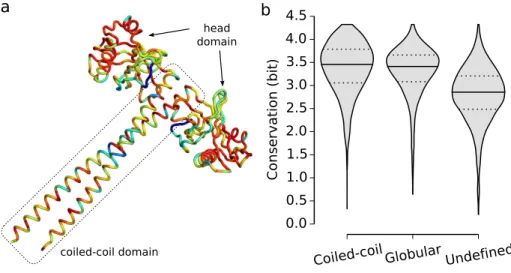
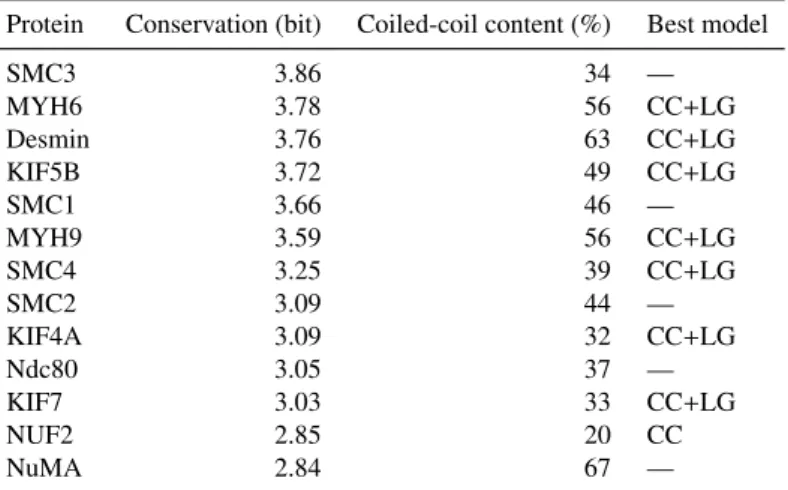
In chapter 2 we analysed the evolutionary properties of coiled-coil sequences. We showed that, despite the underlying simple pattern of hydrophobic and polar residues, coiled-coil sequences are conserved and contain evolutionary relevant information (similar to the globular domains). Yet, the patterns of amino acid substitutions differ from those of globular domains. We developed a coiled-coil

(4)

often leading to different tree topologies. For multidomain proteins, consisting

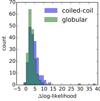
of both coiled-coil and globular domains, model partitioning involving the CC model and a general model yields more likely tree estimates than a single model. Lastly, the new model improves search sensitivity of (sequence similarity-based) homology detection methods for coiled-coil proteins.

Proteins evolve by altering the composition of their primary sequence but also by changing their length. Hence, to complement the analysis of the substitu-tion patterns in coiled-coil domains we also analysed their length evolusubstitu-tion. The number of sequence repeats (in repetitive proteins), and as a consequence protein length, varies across homologues. Yet, given the structural role in the spacer and scaffold formation, we hypothesized, in chapter 3, that the length of coiled-coil

domains is largely conserved in evolution. Indeed, we observed high conser-vation of coiled-coil regions length throughout the tree of life, even when the remaining parts of the protein, including globular domains, change. This length conservation is independent of the conservation of the amino acid composition. It reflects the conservation of the physical length of the domain; contrary to the globular domains, the size of the coiled-coil domains changes proportionally to the change in the sequence length. Length conservation is functionally specific, suggesting that the domain size is constrained by its function.

The remaining chapters focus on the Rab GTPases, a large protein family of closely related proteins that regulates membrane trafficking by providing

speci-ficity to the system. Rabs are short single-domain proteins with a complex evo-lutionary history: They have been subject to multiple general and taxon-specific duplications (and losses). The family structure, its size, and a high level of se-quence similarity pose a challenge for evolutionary inference methods. In chap-ter 4 we present Rabifier2, a new version of a bioinformatic pipeline for Rab GTPase identification and classification. The new Rabifier outperforms the ini-tial version in both the annotation accuracy and speed. It is available as a web service (RabDB, which also includes pre-computed annotations for sequenced eukaryotic genomes) and a stand-alone package. Rabifier is distributed as an open source software, which should foster its further community-driven

(5)

ment.

Mounting evidence suggests that the Last Eukaryotic Common Ancestor (LECA) was a complex organism with many features characteristic of extant Eukaryotes, including a large array of Rab GTPases. Yet, it remains unknown how such elaborate repertoire had emerged. In chapter 5 we analysed the ori-gin of eukaryotic Rabs. Using the new Rabifier pipeline, we predicted putative Rab-like GTPases in Archaea and specifically in Lokiarchaeaon – an archaeal species that contains several eukaryotic signatures, including an expanded reper-toire of small GTPases. The phylogenetic analysis was inconclusive about the position of the archaeal Rab-like proteins within the small GTPase family. Yet, a detailed sequence- and structure-based analysis revealed a strict conservation of Rab-specific motifs that mediate interactions with Rab regulators. A sensitive search revealed that, indeed, putative Rab-binding proteins exist in Archaea, sup-porting the hypothesis that some components of the eukaryotic endomembrane system evolved before LECA.

This thesis focuses on analysing protein properties in the evolutionary con-text. The incorporation of such protein class-specific information can often result in a better inference of the protein evolutionary trajectory. These improvements are, however, not restricted to protein evolution. The presence of characteristic marker proteins in an organism is a strong indicator for the presence of specific cellular processes and structures; conversely, the absence of a protein suggests a missing functionality. Hence, the improved tools for inferring evolutionary re-lationships between proteins should ultimately help to uncover the evolution of cellular components and functions.

(6)

O

sprocessos evolutivos podem ser observados em vários níveis de

organiza-ção biológica. Neste contexto, o trabalho desenvolvido nesta tese centra-se na evolução molecular de proteínas. Apesar de as proteínas serem polímeros li-neares compostos por um conjunto básico de 20 aminoácidos, podem gerar uma enorme variedade de formas e funções. Proteínas que surgiram de um descen-dente comum são classificadas por famílias, que têm geralmente propriedades comuns, incluindo similaridades na sequência, estrutura e função. Vários mé-todos têm sido desenvolvidos para inferir relações evolutivas entre proteínas e classificá-las em famílias. No entanto, esses métodos genéricos são muitas ve-zes imprecisos, especialmente quando propriedades específicas das proteínas li-mitam a sua aplicação. Nesta tese, analisámos duas classes de proteínas que apresentam dificuldades para a análise evolutiva: as proteínas ‘coiled-coil’ – do-mínios de proteínas repetitivas definidas por um motivo simples peptídico ge-neralizado (capítulos 2 e 3) e pequenas GTPases Rab – uma família grande de proteínas muito próximas evolutivamente (capítulos 4 e 5). Em ambos os casos, analisamos as propriedades específicas que determinam a estrutura e função das proteínas, e usamo-las para melhorar a sua inferência evolutiva.

Proteínas ‘coiled-coil’ são domínios do tipo ‘rod’ omnipresentes em todos os seres vivos e que abrangem até 10% de proteínas codificadas num genoma. Estas estão envolvidas em vários processos celulares, onde funcionam como espaçado-res, separando domínios funcionais e/ou pontos de interação, muitas vezes

for-necendo o molde para complexos de proteínas. A resolução da história evolutiva das proteínas coiled-coil permite contribuir para o esclarecimento da evolução de muitos processos e sistemas intracelulares. No entanto, devido à sua baixa complexidade, as proteínas coiled-coil, no contexto da inferência evolutiva são consideradas difíceis: o domínio consiste em múltiplas repetições de um padrão peptídeo simples de sete aminoácidos. Como resultado, os domínios não homólo-gos das coiled-coils podem convergir para uma sequência e estrutura semelhante e as coiled-coils surgiram por várias vezes na evolução de forma independente.

No capítulo 2, analisamos as propriedades evolutivas de sequências de coiled-coils. Mostrámos que, apesar da existência do padrão subjacente de resíduos

(7)

ples, hidrófobos e polares, as sequências em coiled-coil são conservadas e con-têm informação evolutiva relevante (semelhante aos domínios globulares). No entanto, os padrões de substituições de aminoácidos diferem dos domínios glo-bulares. Desenvolvemos um modelo específico de coiled-coil (CC) que reflete esses padrões de substituição. Quando aplicado na reconstrução filogenética de proteínas coiled-coil, supera os modelos gerais, levando muitas vezes a diferen-tes topologias de árvores. Para proteínas com vários domínios, que consistam em domínios coiled-coils e domínios globulares, o particionamento do modelo envolvendo o modelo CC e um modelo geral produz estimativas de árvores com uma maior probabilidade, do que um único modelo. Por último, o novo mo-delo melhora a sensibilidade de busca (baseada em similaridade de sequência) de métodos de detecção de homologia para proteínas coiled-coils.

As proteínas evoluem pela alteração da composição da sua sequência primá-ria, mas também pela alteração do seu comprimento. Assim, para complementar a análise dos padrões de substituição nos domínios coiled-coil, também anali-sámos a evolução do seu comprimento. Entre homólogos varia o número de elementos repetitivos (em proteínas repetitivas), e como consequência, o compri-mento das proteínas. No entanto, dado o papel estrutural como espaçadores e de esqueleto modular, formulamos a hipótese, no capítulo 3, de que o compri-mento dos domínios coiled-coil é largamente conservado na sua evolução. De facto, observou-se uma elevada conservação no comprimento das regiões coiled-coil em toda a árvore da vida, mesmo quando mudam as restantes partes da proteína, incluindo domínios globulares. Esta conservação de comprimento é independente da conservação da composição em aminoácidos. A conservação do comprimento físico dos domínios coiled-coils varia proporcionalmente à al-teração no comprimento da sequência em oposição ao observado em domínios globulares. A conservação do comprimento é específica da funcionalidade, o que sugere que o tamanho do domínio é limitado pela sua função.

Os restantes capítulos focam as Rab GTPases, uma família numerosa de pro-teínas evolutivamente muito próximas, que regulam o tráfico membranar, forne-cendo especificidade a este sistema. As Rabs são proteínas de domínio único com uma história evolutiva complexa: foram sujeitas a duplicações (e perdas) gerais múltiplas e taxonomicamente específicas. A estrutura desta família, o seu

(8)

versão atualizada de uma cadeia de comandos bioinformáticos para identificação e classificação de Rab GTPases. O novo Rabifier supera a versão inicial, tanto pela precisão na anotação como em velocidade. Está disponível como um ser-viço web (RabDB, que também inclui anotações pré-analisadas para os genomas eucarióticos já sequenciados) e um pacote ‘stand-alone’. O Rabifier é distribuído como um software de código aberto, o que visa promover o seu desenvolvimento pela da comunidade de utilizadores.

Evidências crescentes sugerem que o último ancestral comum de todos os eucariotas (do inglês LECA) era um organismo complexo com muitas caracte-rísticas típicas dos eucariotas atuais, incluindo uma grande variedade de Rab GTPases. No entanto, continua a ser um mistério como terá emergido tal com-plexidade. No capítulo 5, analisamos a origem das Rabs eucarióticas. Usando a versão actualizada do Rabifier, previmos potenciais GTPases do tipo Rab em Archaea e, especificamente, no Lokiarchaeaon – uma espécie de Archaea que contém várias assinaturas eucarióticas, incluindo um repertório expandido de pequenas GTPases. A análise filogenética foi inconclusiva sobre a posição das proteínas Rab-like de Archaea, dentro da família das pequenas GTPases. No entanto, uma análise detalhada baseada em estrutura e sequências revelou uma conservação estrita de motivos específicos de Rab que medeiam as interações com os reguladores Rab. Uma pesquisa fina revelou que, de facto, existem po-tenciais proteínas de ligação a Rabs em Archaea, suportando a hipótese de que alguns componentes do sistema endo-membranar eucariótico evoluíram antes do LECA.

Esta tese centra-se na análise de propriedades de proteínas no contexto evo-lutivo. A incorporação de informações específicas de classe de proteínas resulta numa melhor dedução da trajetória evolutiva das proteínas. Estas melhorias, no entanto, não são restritas à evolução de proteínas. A presença de proteínas de características específicas num organismo são um forte indicador para a eventual presença de processos e estruturas celulares específicas. Por outro lado, a ausên-cia de uma proteína sugere uma funcionalidade perdida. Em última análise, a disponibilização de melhores ferramentas para a aferição de relações evolutivas

(9)

entre as proteínas deverá contribuir para a descoberta da evolução dos compo-nentes e funções celulares.

(10)

(11)

C

hapter

1

(16)

P

, linear polymers built by a limited set of amino acids, gen-erate an enormous variety of forms and functions. Many methods have been developed to describe and catalogue this diversity. Yet, their performance is often limited by neglecting protein-specific properties. In this chapter, we introduce concepts related to protein classification by evolutionary inference. We first review and discuss the basic methods used in molecular evolution, that is, putative homology detection using sequence similarity as a proxy, multiple sequence alignments, and phy-logeny reconstruction, followed by their applications and a description of automated methods. In the following section, we describe properties that define the accessible space of protein evolution. The available space of protein structures is virtually infinite, yet, the observed proteins cover only its tiny fraction. It is a result of constraints imposed on the sequence, necessary to preserve protein structure and function. The presence of such restraints, specific to each protein, alters the information content of a sequence that can be used for evolutionary inference. We conclude by describing two ‘difficult’ protein classes, challenging for an evolutionary

analysis, that are the objects of studies in the remainder of this thesis.

(17)

1.1. Introduction 3

1.1 Introduction

P

roteinsare fundamental building blocks of life. They are involved in

virtu-ally all biological processes, their function ranges from catalyzing diverse biochemical reactions to providing the internal structure of the cell. Since their discovery, proteins are at a main focus of the molecular biology research. The ar-rival of the insulin sequence in early 1950s (Sanger and Tuppy 1951a; Sanger and Tuppy 1951b), the first full protein to be ever sequenced, demonstrated that proteins can be characterized by a linear combination of amino acids, the building blocks of every protein (reviewed by, Stretton 2002). In the following years, Sanger and co-workers obtained insulin sequences from a few different

species allowing for a comparative sequence analysis, which revealed that the interspecies amino acid differences are confined to a single short region (Harris

et al. 1956). Since then, millions of proteins have been sequenced1_{; for example,}

more than 40 million unique proteins have been deposited in the UniProt data-base (UniProt Consortium 2015). Continuous growth in the amount of sequence information allowed for comparative protein analyses and, given sequences of related proteins from different species, sequence-based evolutionary analyses

(molecular traits can be used to reconstruct phylogenetic trees similarly to the morphological features). In this chapter, we review the literature and describe the advances in the field of molecular evolution with a special focus on protein evolution. We first describe the importance of the evolutionary analysis and the common methods used for the evolutionary inference. We then focus on pro-tein properties and discuss how they can influence the analysis. We conclude the chapter by describing problems and challenges in evolutionary inference and discuss two cases of ‘difficult’ protein classes, which are the subject of the

re-maining chapters.

1.1.1 Biological classification: from organisms to molecules

Humans have always been intrigued by the natural diversity of living things and tried to catalogue this diversity by describing relationships between organisms.

1_{In contrast to the early approaches, protein sequences are generally predicted from the}

(18)

The first major attempt to classify living things was proposed by Aristotle. He grouped organisms based on their common features, for example, he separated animals into two groups: ‘animals with blood’ and ‘animals without blood’, he further divided the former into ‘live-bearing’ and ‘egg-bearing’. These groups were arranged into a ranked linear structure based on their complexity of struc-ture and function, scala naturae(‘ladder of life’), organisms ranked higher on

the ladder showed greater ability to move and sense. The first modern classifica-tion system of living things was proposed by Carl Linnaeus in the 18th century. In this system, each organism is represented by a list of ranked terms: Organ-isms that share morphological similarities are grouped together into ataxonof a

given taxonomic rank; low-ranked taxa are then grouped into higher level taxa to form a nested hierarchical structure, ataxonomy(reviewed, e.g., by Sivarajan and

Robson 1991; Ohl 2007). A major breakthrough in the biological classification system came with the inception of the evolutionary theory. The incorporation of the evolutionary theory into the biological classification created a modern system based on the evolutionary relationships between species (both living and extinct) rather than similarities in morphology. The theory introduced the temporal di-mension to the taxonomy, which allowed asking questions not only about how organisms are related to each other but also how distant they are, that is, when (and what) was their common ancestor. In this system, species that share a com-mon ancestor are organized into groups, calledclades, that form a hierarchical

structure – a tree describing the evolutionary history of this group of organisms (reviewed, e.g., by Queiroz and Gauthier 1994).

Predicting true evolutionary relationships between organisms using compara-tive morphology can be especially challenging, for example, due to the presence of analogous morphological traits (outcomes of convergent evolution) that group together unrelated species. The recent revolution in molecular biology offers a

(19)

1.1. Introduction 5

was inconclusive about panda’s classification with bears, raccoons or as a sepa-rate family), placing it at the base of the Ursidae family (O’Brien et al. 1985).

The use of sequence data in building the biological classification of the liv-ing thliv-ings have largely replaced morphological information; it also marks the in-ception of a new discipline, molecular evolution, whose applications go beyond reconstructing species histories. Molecular evolution is an area of evolutionary biology that studies evolutionary changes at the DNA, RNA and protein level and the mechanisms that drive those changes (Li 1997). Proteins, similarly to species, can be classified into hierarchical groups based on their common ances-try, which is usually predicted from sequence similarities (related proteins often share other similarities, e.g., structure, function). However, inferring protein evo-lutionary histories is often challenging, due to a limited amount of information present in the sequence and complex relationships between proteins (sequences can arise not only by speciation but also by duplication events, they can be lost from a genome or incorporated by horizontal gene transfer; reviewed, e.g., by Koonin 2015). Hence, accurate methods are required to recover true relation-ships between proteins.

1.1.2 Motivation

(20)

dif-ferent protein classes, which impose specific constraints on sequence evolution (e.g., intrinsically disordered proteins, Brown et al. 2010).

In this thesis, we analysed how specific molecular properties influence pro-tein evolutionary trajectory by examining two propro-tein classes that challenge the existing methods for molecular evolution: the coiled-coils – widespread pro-tein domains formed by a simple repetitive peptide motif; Rab small GTPases – closely related proteins forming a large family with a complex structure. Based on this analysis, we developed new tools and proposed changes to the existing methods that improve homology detection and evolutionary analysis of coiled-coil proteins and Rab GTPases. We used some of these developments to study the origin of the eukaryotic endomembrane trafficking system.

1.2 Methods of molecular evolution

The methods of molecular evolution are used to describe the evolutionary process that generates the observed molecular variation at the sequence level. A common goal of an analysis is to identify proteins that originated from a common ancestor (homologues) either in the species of interest or in all available sequence data. Yet, even if the objective is more specific, detection of homologous sequences is the necessary initial step, which determines the accuracy of the consecutive steps of the analysis. In fact, each step of the analysis pipeline should be evaluated, as any error will propagate to the subsequent steps of the pipeline and influence the final result (e.g., Anisimova, Liberles, et al. 2013).

The classical phylogenetic analysis pipeline is usually divided into four steps (Holder and Lewis 2003; Anisimova, Liberles, et al. 2013): identification of ho-mologous sequences, construction of a multiple sequences alignment, tree es-timation, and hypothesis testing on the constructed phylogeny. In this thesis we mainly focus on two of these steps, that is, identification of the homolo-gous/orthologous sequences and estimation of phylogenetic trees. We develop

(21)

1.2. Methods of molecular evolution 7

phylogenetic trees can be constructed based on sequences of morphological char-acters, e.g., Lewis 2001).

1.2.1 Sequence search

The goal of the first step of an evolutionary analysis is the identification of pu-tative homologous sequences. Proteins related by the common descent are ex-pected to share common features, including similarities at the sequence level. The premise of higher sequence similarity between related than unrelated pro-teins is at the core of the homology detection methods. Arguably the most popu-lar method is BLAST (Basic Local Alignment Search Tool, Altschul et al. 1990; Altschul 1997; Camacho et al. 2009), a very fast search tool based on pairwise local alignments, which allows scanning large sequence databases. However, the algorithm loses sensitivity at larger evolutionary distances (high sequence divergence); this deficiency can be improved by using multiple homologous se-quences as a query instead of relying on pairwise comparisons (Park et al. 1998; Madera 2002). Such sequences can be identified in an iterative search, where the initial search detects similar sequences used to build a scoring profile that is subsequently used to detect more distant sequences (e.g., PSI-BLAST, Altschul 1997). Even more sensitive methods (Madera 2002) use profile hidden Markov models (pHMMs) that combine probabilities of both character substitutions and insertion/deletion events at each position of a sequence to improve search

accu-racy (Krogh et al. 1994; Eddy 1996; Eddy 1998). This approach for similarity search has been implemented in, for example, SAM (Hughey and Krogh 1996; Karplus et al. 1998) and HMMER (http://hmmer.org). These similarity-based

methods identify putative homologues. Homologues are related to one another in several ways (see fig. 1.1) and methods based solely on sequence similarity comparisons can predict some of these relationships.

(22)

Gold-human ✁

human ✂'

platypus ✂

x

mouse ✁

platypus ✁

human ✂

mouse ✂

x

in-paralogues

out-par

alogues

co

-orthologues

orthologues

homologues

x

duplication

loss

Fig. 1.1.Evolutionary relationships between genes descended from a common ancestor

(homologues). Orthologues are genes that evolved from their most recent an-cestor by speciation; paralogues evolved from a duplication event (Fitch 1970). Genes are defined as out-paralogues if they duplicated before a speciation event and in-paralogues if a duplication occurred after the speciation. In-paralogues are collectively orthologous (co-orthologues) to other genes related by specia-tion. For a more comprehensive description of homologous relationships see, for example, a review by Koonin (2005).

ing (2001) reported that the closest BLAST hits are often not the nearest neigh-bors on a phylogenetic tree. Such a situation can result from a difference in

func-tional constraints and rates of evolution across homologous genes (e.g., Koonin 2005; Studer and Robinson-Rechavi 2009). Despite these problems, sequence-similarity-based methods are commonly used for orthology prediction due to their speed and relatively good performance (e.g., Hulsen et al. 2006; Altenhoff

and Dessimoz 2009; Wolf and Koonin 2012). For example, in the popular

bidi-rectional best hits(BBH or reciprocal best hits, Overbeek et al. 1999) approach,

a pair of sequences in two different genomes is considered orthologous if they are

more similar to each other than to any other sequence in the other genome. BBH allows finding probable pairs of orthologues, yet, an additional step is required to obtain a group of orthologous sequences from multiple species: an all-against-all BBH search generates orthologous pairs that are subsequently linked to form clusters of orthologues (Tatusov 1997).

(23)

meth-1.2. Methods of molecular evolution 9

ods (reviewed by Kristensen et al. 2011). They offer several advantages over

tree-based methods (e.g., Kuzniar et al. 2008). They are usually much faster and easier to automate, which makes them especially useful for large datasets. Being based on pairwise comparisons, they avoid errors associated with the construc-tion of multiple sequence alignments, gene, and species trees. Yet, similarity-based methods have several limitations. For example, BBH is susceptible to taxon-specific gene loss, where it can erroneously assign orthology relationships (e.g., Dessimoz et al. 2006; Scannell et al. 2006); for instance, in the example presented in figure 1.1, genes from the mouse and platypus pair would be clas-sified as orthologous (as the most similar hits in both genomes) due the loss of complementing paralogues. Similarly, BBH also fails to identify many ortho-logues in duplication-rich taxa (e.g., Dalquen and Dessimoz 2013). Heuristic similarity-based methods are generally more suited for comparative studies; they are unable to provide a detailed description of the evolutionary process that gen-erated observed sequences.

(24)

number of false hits, yet, it also reduces the search sensitivity, especially when the low-complexity regions span a significant part of the protein.

1.2.2 Sequence alignment

Given a set of candidate homologous sequences, the next step in the analysis is the construction of a multiple sequence alignment. An alignment of biological se-quences is formed by inserting gaps of varying length into sese-quences to form an array where each column contains homologous residues: a given column is a hy-pothesis that all residues at this position descended from a common ancestor. The problem of finding an optimal multiple sequence alignment (MSA) can be solved with a dynamic programming algorithm. However, the computational complex-ity grows exponentially with the number of sequences,_O(ln) wherelis the

(25)

procedure is repeated until convergence (e.g., Katoh 2002; Edgar 2004). Sev-eral other methods have been proposed to improve MSA accuracy, for example, T-Coffee (Notredame et al. 2000), MUSCLE (Edgar 2004), Probalign (Roshan

and Livesay 2006), Clustal Omega (Sievers et al. 2014). These methods differ in

the accuracy of the estimated MSA and computation speed (slower methods usu-ally produce more accurate alignments). In this thesis, we mainly used MAFFT (Katoh and Standley 2013), a computationally efficient method that offers high

MSA accuracy (Ahola et al. 2006; Nuin et al. 2006; Sievers et al. 2014; Thomp-son, Linard, et al. 2011).

Protein structure is generally better conserved than sequence. Hence, the pro-cess of sequence alignment may benefit from including structural information. An experimental structure(s) of a sufficiently similar protein can serve as a

tem-plate for the alignment; gap insertions at structure-altering positions should be rejected. However, if direct experimental data is unavailable, the alignment esti-mation may be reinforced with inforesti-mation from secondary structure predictions (e.g., PSIPRED, Jones 1999) and 3D structures of homologous proteins (3DCof-fee, O’Sullivan et al. 2004); both sets of information are used in PROMALS3D (Pei et al. 2008).

Widely used aligners find an optimal MSA by maximizing similarities be-tween sequences for a given set of scoring parameters (substitution and gap penalty). However, such alignment may not reflect correct evolutionary relation-ships between sequences. A different class of aligners referred to as

(26)

Multiple sequence alignments are central to many sequence-based analyses including phylogenetics, domain characterization and motif search; the outcome of these analyses is strongly dependent on the accuracy of the alignment. Hence, it is important to determine the overall alignment quality and find unreliable, highly variable often gap-rich, regions. In fact, removing such unreliable posi-tions often leads to an improvement in the downstream analysis (Talavera and Castresana 2007). Different methods have been developed to analyse sequence

alignments (measure its quality and robustness) and find low-quality regions (for example, Castresana 2000; Capella-Gutierrez et al. 2009; Wu et al. 2012; Sela et al. 2015).

1.2.3 Phylogeny reconstruction

The goal of the phylogenetic reconstruction is to find the most probable hypothe-sis describing the evolution of a set of sequences – the phylogenetic tree. In this section, we briefly describe the most popular methods for phylogenetic inference and discuss their advantages and disadvantages.

A simple approach to determine the relationships between sequences is to use the maximum parsimony optimality criterion. The maximum parsimony method searches for the shortest possible (most parsimonious) tree, that is a tree that accounts for the fewest possible changes between sequences (Fitch 1971). Al-though it is easy to count the number of changes for a given tree topology, the method requires exploring the entire topology space to find the most parsimo-nious tree, which is impractical for large alignments2_{. This method is}

conceptu-ally simple and does not require any model of molecular evolution. This, how-ever, may be problematic as all substitutions have equal weight, which in many cases can produce wrong results. Due to its design, the method always finds the shortest tree, often underestimating the true number of substitutions between se-quences (multiple substitutions can occur at a single position), especially at long evolutionary distances (Saitou 1989).

A different class of methods is based on pairwise distances between sequences.

2_{The number of tree topologies grows exponentially with the number of sequences. Exhaustive}

(27)

In the simplest form, the distance can be expressed as the number of residue dif-ferences, either nucleotide or amino acid, between two sequences. This approach transforms a sequence alignment into a symmetric matrix of pairwise distances. The distance matrix can be subsequently processed with widely used clustering algorithms (e.g. UPGMA (Sokal and Michener 1958), Neighbor-Joining (Saitou and Nei 1987)) to produce a hierarchical structure – a phylogenetic tree represent-ing the relationships between the species. The branch lengths of the constructed tree should approximate the pairwise distances of the distance matrix. Neighbor-Joining (NJ) is a fast algorithm, it is especially suitable for large alignments or for a bootstrap analysis, its execution time is proportional to the cube of the num-ber of sequences, O(n3) (Studier and Keppler 1988). Distance based methods

have several problems and limitations. For example, the NJ algorithm does not guarantee to construct tree branches with non-negative lengths if the distance matrix is non-additive (Kuhner and Felsenstein 1994). NJ does not explore the available topology space and compare different trees, compared to the methods

described below, its outcome is a single tree. Hence, it is not possible to analyse other high-scoring trees that could support an alternative hypothesis about the homologous relationships between sequences (see, e.g., Gascuel and Steel 2006, for a review about NJ).

Assigning equal scores to all residue changes may result in incorrect phylo-genies. The observed number of changes is often smaller than the real number, especially at longer evolutionary distances or higher rates of evolution: mul-tiple substitutions occurring at the same position in the sequence result in an underestimation of the observed distance between sequences (Jukes and Can-tor 1969). Both the stationary amino acid frequencies in protein sequences and the substitution rates between them differ for each amino acid according to its

chemical and physical properties. For example, substitutions within polar, neg-atively/positively charged, hydrophobic and aromatic groups are less prone to

(28)

that describe probabilities (rates) of changes for each pair of amino acids, or nu-cleotides in the case of DNA (some models also exist for codon substitutions, see e.g., Goldman and Yang 1994). Box 1.1 describes substitution models in a greater detail. Substitution models can be used to compute distances between sequences (Felsenstein 1989) to account for the type of the observed changes, which should result in a more accurate estimation of the real evolutionary dis-tance.

The probabilistic methods of phylogenetic inference, Maximum Likelihood (ML) (Felsenstein 1981) and Bayesian inference (Rannala and Yang 1996; Yang and Rannala 1997), offer many improvements over maximum parsimony and the

distance-based methods. Yet, the improvements provided by these methods come at a much greater computational cost (only the recent growth of computational power enabled the inference of large phylogenies in reasonable time). In the ma-jority of cases, the probabilistic methods provide a more accurate estimate for phylogenetic trees (see, e.g., Kuhner and Felsenstein 1994; Spencer 2005; Og-den and Rosenberg 2006). ML and Bayesian methods infer phylogenetic trees di-rectly using information contained in the sequence alignment in contrast with the distance methods. As a result, no information is lost in the process of data trans-formation from an alignment to pairwise distances between sequences. These methods define probabilistic frameworks that are used to find the best tree for the given alignment by exploring the available topology space. Every inspected tree is scored, so the outcome of the analysis is, in fact, a collection of trees, each with a confidence value assigned to it. Maximum Likelihood and Bayesian meth-ods explore the parameter space to find the best set of parameters for the given data. Tree topology and branch lengths are a subset of these parameters, arguably the most interesting outcome of the analysis. However, other parameters must be provided (or derived from the data) to compute the phylogeny. The crucial set of parameters describe expected residue frequencies and the probabilities of residue substitutions; it is defined by substitution models (Box 1.1). Many mod-els have been defined for different protein classes to obtain optimal phylogenetic

(29)

a wrong hypothesis – Eukaryotes being a sister group to Archaea (Rinke et al. 2013). This demonstrates the importance of adjusting model parameters to ac-count for specific sequence properties. Some additional parameters can also be specified to improve inference. For example, positions in the alignment can be divided into groups by their rate of evolution to account for the difference in

substitution rates along the sequence; this is usually accomplished by defining several categories following the gamma distribution whose shape parameter (α)

can be co-estimated from the data (Yang 1996).

Box1.1 Models of molecular evolution

Models of molecular evolution, or substitution models, describe the pro-cess where one character replaces another (substitution) in a sequence of characters of a given alphabet (e.g. nucleotides, amino acids). The mod-els are usually represented in a form of a square transition matrix where each elementai j describes the probability (rate) of change from the

char-acterito j. The size of the matrix equals to the length of the alphabet.

Substitution models belong to two categories: mechanistic and empirical. Parameters of mechanistic models are derived from the knowledge about the fundamental processes that guide sequence evolution. Conversely, parameter values of empirical models are estimated from alignments of real sequences, without considering factors that led to the observed sub-stitutions. A simple mechanistic model for DNA may define two parame-ters that distinguish rates of transitions and transversions (Kimura 1980). In the Maximum Likelihood framework, the values of both parameters are simultaneously estimated with the parameters for tree topology and branch lengths to maximize the probability of the model for the given data. Mechanistic models are mostly defined for DNA and codons; at the protein level, evolutionary processes are usually described with em-pirical models. The first widely used model of amino acid substitution, PAM (Point Accepted Mutation), was proposed by Dayhoffet al. (1978).

(30)

informa-tion from sequences separated by longer evoluinforma-tionary distances. Recent methods use the Maximum Likelihood framework to estimate substitu-tion rates from large datasets covering different evolutionary distances.

For example, the widely used general WAG (Whelan and Goldman 2001) and LG (Le and Gascuel 2008) models. Some models were designed to address specific conditions, for example, a model for proteins encoded by the mitochondrial DNA (Adachi and Hasegawa 1996) or even specifically mitochondrial proteins from Arthropoda (Abascal et al. 2006).

Selecting a good model for given sequences can be difficult.

How-ever, it is possible, within the likelihood framework, to compare models and select one that provides the best fit to the data. This can be achieved by comparing likelihoods and the number of parameters for each model using measures like AIC (Akaike information criterion, Akaike 1974) or BIC (Bayesian information criterion, Schwarz 1978). The assumption of independent evolution at each position in the sequence allows assign-ing multiple best-fittassign-ing models to a protein (an approach named model partitioning) to reflect a difference in the evolutionary process between

protein regions.

1.2.4 Applications

The final result of the phylogenetic reconstruction is an evolutionary tree – a hypothesis describing the evolutionary process that generated the observed se-quences from the common ancestor. Given the reconstructed gene/protein

phy-logeny and the corresponding species tree, it is possible to map homology re-lationships (orthology, paralogy) between sequences in the process of tree rec-onciliation (Goodman et al. 1979). In the parsimony framework, the process minimizes the number of gene duplications and losses necessary to inscribe the gene tree into the species tree (this and other algorithms for tree reconciliation are described by Doyon et al. 2011).

Arguably the most common application of phylogenetic methods is the recon-struction of species and gene/protein trees. Yet, these methods allow addressing

(31)

Holder and Lewis 2003, for more examples).

Trees inferred with Maximum Parsimony, Maximum Likelihood or Bayesian methods (i.e. methods operating directly on sequence information, character-based methods) contain estimates of the ancestral state at each of the internal branches. This information presents an interesting opportunity to infer sequences of ancient proteins. In fact, multiple reports describe not only theoretical predic-tions but synthesis, or ‘resurrection’, of ancient proteins, based on the phyloge-netic reconstruction, and subsequent exploration of their properties and function. For example, Gaucher et al. (2008) showed higher thermostability of ancient elongation factors, which coincided with Earth hotter environment. For more examples and additional information see Thornton (2004).

Multiple substitution models can be compared to determine which one is the best fit for the given sequence data. This approach can also be used for hy-pothesis testing about the data. For instance, it is possible to detect selection by comparing two nested models where one allows for sites under positive selec-tion, another does not. If the more complex model, which includes selecselec-tion, is substantially better that the simpler one (as measured with likelihood ratio test, AIC, or BIC) it is possible to conclude that some sites are under selection in the analysed sequence (for more information see, e.g., Huelsenbeck et al. 1997; Anisimova, Bielawski, et al. 2001; Yang 1998). For example, Gibbs and Rossiter (2008) showed that venom coding genes in rattlesnakes are rapidly evolving by positive selection; similarly, Bulmer and Crozier (2006) described positive selec-tion in termite immunity genes.

1.2.5 Automatic methods

The traditional approach to the evolutionary analysis of sequence data involves extensive manual interaction: each step (i.e. homology detection, sequence align-ment, tree reconstruction) is run and validated by a human expert. The outcome of such approach is expected to be more accurate than the result of an automatic analysis. Yet, it often depends on subjective choices and is difficult to reproduce.

(32)

proteins across hundreds of species. Many tools and databases, which differ in

the applied methodology, taxonomic sampling, and performance, have been de-veloped over the years. These methods can be divided into two categories: graph-based methods that cluster orthologues graph-based on their sequence similarities (e.g., COG, Tatusov (2000); EggNOG, Powell et al. (2014)) and phylogenetic tree-based methods (e.g., PhylomeDB, Huerta-Cepas et al. 2014); hybrid approaches combine both graph- and tree-based methods on different stages of the pipeline

(e.g., Ensembl Compara, Cunningham et al. 2015, generates sequence clusters based on a BLAST-similarity-search graph, which are subsequently aligned and used to build phylogenetic trees; finally the gene trees are reconciled with a species tree to map duplication evens). Automatic methods allow annotating full genomes, which is especially important given the recent developments in the DNA sequencing technologies that greatly reduce the effort and time of obtaining

new genomes, often making the analysis and annotation the limiting step.

1.3 Protein space, constraints, and information content

The pipeline, described in the former section, provides a general framework for a phylogenetic analysis. Yet, the details of an analysis may differ depending on

specific properties of a given protein. In this section we will describe factors that may influence the evolutionary trajectory of a protein and as a consequence require adjustments to the phylogenetic analysis.

1.3.1 Protein space

Theoretically, given that every position in a sequence can be occupied by one of the 20 amino acids, the number of possible proteins grows exponentially with the length (n) of the polypeptide chain (20n). For example, a relatively short peptide

of 100 residues can be built by 20100_{, or approximately 1}_.₂₇_×₁₀130_{, di}_ff_erent

(33)

1.3. Protein space, constraints, and information content 19

these factors influence protein evolution and, as a consequence, the challenges they present to the evolutionary analysis. Yet, first, we describe the properties of the observed protein space.

Proteins are composed of domains, continuous stretches of amino acids with distinct structure, function and evolutionary history. A simple protein may con-sist of only a single domain, yet, multi-domain proteins are more common (Te-ichmann et al. 1998; Vogel et al. 2004). The same domain may exist in multiple different proteins, its combinations with other domains form uniquedomain

ar-chitectures. Different architectures are formed by duplication, divergence, and

recombinations of existing domains (reviewed by Vogel et al. 2004). New protein functions can arise from domain combinations, which differ from the functions of

single-domain proteins (Bashton and Chothia 2007). Domains are classified into families: a domain family contains small single-domain proteins and fragments of larger proteins that have arisen from the common ancestor. The distribution of domain family sizes in individual genomes (and larger taxonomic groups) is highly skewed, it follows the power-law distribution: a few families have many members, the remaining families have only a few members. The family size dis-tribution can be explained by a stochastic model of domain birth (duplication) and death (loss) (see, e.g., Qian et al. 2001; Karev et al. 2002).

Most proteins require being properly folded into a three-dimensional struc-ture in order to perform their function and interact with their partners (only 2-3% of prokaryotic and 20-30% eukaryotic proteins contain long intrinsically disor-dered regions, Dunker et al. 2001; Ward et al. 2004; Schlessinger et al. 2011). Despite the enormous size of the universe of possible protein structures, a sur-prisingly small space is used by nature. At the time of writing, the PDB database (Protein Data Bank, http://www.rcsb.org) contains 36642 unique structures3, yet,

the total number of structural folds is estimated only in the order of thousands (Wolf, Grishin, et al. 2000; Govindarajan et al. 1999) (for more information con-cerning protein structural classification see Box 1.2). This implies that proteins are restricted to a limited space of structural folds, which largely constrains their sequence evolution. Indeed, the analysis of the available protein structures shows that the observed protein folds occupy only four regions of the sparsely populated

3_{Non-redundant structures at 95% of sequence identity; at 70% the number of unique structures}

(34)

protein structure space (Hou et al. 2003). These regions roughly correspond to the four classes defined, in the SCOP classification, by their secondary structure composition: all-α, all-β,α+β,α/β(see Box 1.2).

Box1.2 Protein structural classification

Proteins are classified into different levels of organization that reflect

their structural and sequential similarities and evolutionary relatedness. The SCOP (Structural Classification of Proteins) classification system (Murzin et al. 1995), based on proteins with known three-dimensional structures, provides a comprehensive description of structural and evolu-tionary relationships between proteins. It classifies proteins into a number of hierarchical levels, where family, superfamily, fold, and class are the principal ones.

1. Family: Proteins classified at the family level are clearly

evolu-tionary related. They share high sequence similarity, the pairwise sequence identity is usually greater than 30%. However, in some cases, despite very low pairwise sequence similarity, proteins are classified into a family based on similar function and high struc-tural similarity, for example, globins.

2. Superfamily: Proteins are not necessarily related at the superfamily

level. Pairwise sequence similarities are low, yet, similarities in structure and function suggest a common origin.

3. Fold: Proteins share a common fold if they have the same major

secondary structures in the same arrangement and the same topo-logical connections. However, proteins with the same fold may differ in peripheral secondary structure elements, which may

(35)

conditions favoring certain structural arrangements.

4. Class: At the class level groups are formed based on the secondary

structure content and organization, that is, proteins formed only by

α-helices (all-α), only byβ-strands (all-β), bothα-helices andβ

-strands that are largely segregated (α+β), and interspersed (α/β).

The SCOP classification is used by other services, for example, the SU-PERFAMILY database (Gough et al. 2001) that builds hidden Markov models based on SCOP superfamilies to annotate proteins in more than 2400 genomes. Alternative systems of protein structural classification exist, for example, the CATH hierarchic classification of protein domain structures (Orengo et al. 1997).

1.3.2 Structural constraints in protein evolution

Evolutionary processes that govern protein evolution are constrained by struc-tural requirements of a protein to perform its function. Constraints differ not

only across protein families but also between different regions of a single

pro-tein. They depend on multiple factors that vary along the sequence (e.g., solvent accessibility, local structure of the peptide chain) that define a local environment of each residue in a folded protein, determining amino acid mutability at that position (Overington, Johnson, et al. 1990; Overington, Donnelly, et al. 2008).

Regions of an amino acid sequence assemble into elements of secondary structure that interact with each other, folding into a native, three-dimensional protein structure. The most common secondary structure elements are classi-fied into four types (α-helices, β-sheets, loops, and coils) based on the spatial

arrangement of the chain, defined by the dihedral angles of the peptide bond. The space of energetically allowed dihedral angles differs for each amino acid;

(36)

inference, for example, Thorne et al. (1996) developed a model that describes the organization of the secondary structure along the sequence and substitution rates for each structure.

Another factor that defines a local environment of an amino acid is solvent accessibility. The rate of amino acid substitutions greatly varies between pro-tein regions depending on their exposition to the solvent. The lowest rate of substitution is in the solvent-inaccessible core of a protein and the most con-served residues are polar residues buried inside the core (Overington, Donnelly, et al. 2008). Information about solvent accessibility enriches the description of protein local environments; it can be used to improve models of protein evolu-tion. For example, Goldman, Thorne, et al. (1998) extended the earlier approach (Thorne et al. 1996) to not only account for the difference in substitution patterns

between secondary structure elements but also for the solvent accessibility of these elements.

(37)

(Worth and Blundell 2009).

Evolutionary constraints on protein structure are a consequence of its func-tion: proteins need to fold into native three-dimensional structures to perform their functions. However, specific functions (for example, catalytic activity or interaction with other molecules) impose additional constraints on local amino acid properties. Residues that are closer in space to the functional site are more conserved (Chelliah et al. 2004). Proximity to the active site poses an additional constraint on amino acid substitutions; it should be included in the description of local environments.

Ultimately, the constraints that define a local environment, and limit amino acid substitutions, are a product of the secondary structure, solvent accessibility, features of the global protein architecture and functional requirements. A good characterization of local environments may improve identification and classifica-tion of protein family members, or help in predicting important regions (inter-actions, catalytic activity) of unknown proteins. Using entire information about amino acid local environments in an evolutionary analysis of a protein family may not be practical or even possible. However, understanding specific con-straints of a protein or, at least, its regions may improve the analysis.

1.3.3 Information content

Sequences of DNA, RNA and proteins are carriers of biological information. The amount of information, or informativeness, can be measured in different

ways. However, one of the most commonly used descriptions comes from the information theory developed by Claude Shannon (Shannon 1948) that measures information in terms of entropy of an object4_{. Entropy describes an uncertainty}

(how much is not known) about a state of an object (a random variable); it is defined as a weighted sum of log-probabilities of possible states of a random variable5_.

4_{A di}_ff_{erent measure (Kolmogorov complexity) defines information as the length of the} short-est computer program that produces the observed sequence.

5_{Entropy is a subjective measure that depends on a given definition of the state space of the}

(38)

H(X)=₋

n

X

i=1

p(xi) logp(xi) (1.1)

Conversely, information describes the amount of knowledge about the ob-ject’s state; it allows to make a better prediction, than by chance, about the state of a random variable. It is defined as the difference between the maximal entropy

(i.e. when nothing is known about the object, before the measurement) and the observed remaining entropy (after the measurement).

I =Hmax−H(X) (1.2)

Information theory found many applications in analysing biological sequences. For instance, the difference in information patterns along a genome (horizontal

information) can be used to distinguish coding from non-coding regions (Grosse et al. 2000). Sequence information can also be used to improve the sequence assembly process by clustering sequences bases on their mutual informativeness (Otu and Sayood 2003). Here, we focus on the sequence information across genomes (vertical information) that describes the evolutionary process.

Per-site information content can be calculated given an alignment of homol-ogous sequences. The resulting profile provides a measure of conservation of each position and is commonly used to construct sequence logos (Schneider and Stephens 1990): a graphical representation of the alignment, where each position is represented as a character stack, the height of each character corresponds to its frequency at a given position and the height of the entire stack to the position’s informativeness. Sequence logos are widely used in analysis and visualization of binding sites, conserved motifs, protein domains, and many other applications.

A certain level of sequence conservation is necessary for an accurate detec-tion of putative homologous sequences and to construct a sequence alignment. It is also necessary for phylogenetic inference, for example, to avoid tree recon-struction artifacts like long-branch attraction (Felsenstein 1976). Yet, sequence conservation is not a perfect measure of the sequence informativeness for a phy-logenetic analysis; some divergence is necessary to determine relationships be-tween sequences. The global difference is the rates of evolution have been used to

(39)

highly conserved genes for ancient events and rapidly evolving for recent events. Yet, the choice of those genes is often arbitrary, since the informativeness of the genes is not quantified.

Townsend (2007) proposed a measure of phylogenetic informativeness: the phylogenetic power to resolve evolutionary relationships at a given time during evolution of a gene. A sequence needs to have parts that evolve at an appropri-ate pace to resolve a branching pattern at a given time. Positions evolving too slowly are unlikely to change on a given short internal branch, conversely, po-sitions that are evolving too fast are likely to change also in one, or more, of the descendant clades. Hence, the positions with the highest informativeness for a given inner branch evolve at optimal intermediary rates that maximize the probability of a change occurring at the branch and not at the tips. Phylogenetic informativeness is ultimately a measure of the rate of character change at a given time. For instance, codon positions differ in the substitution rates, the third (most

variable) position is the most informative about the recent events, first and sec-ond about more ancient events (Townsend 2007). Phylogenetic informativeness differs from the branch support estimates (e.g., bootstrap values, posterior

prob-ability); it measures the power of a set of characters to define clades at a given evolutionary time, it does not show how much data support a particular clade. The amount of phylogenetic information at a given time may also reveal if a short branch is a result of a rapid radiation event or lack of appropriate data. High in-formativeness and low branch support indicate rapid radiation, conversely, both low informativeness and low support suggest insufficient data to resolve a given

polytomy.

(40)

1.4 Problems, limitations, and challenges in studying

pro-tein evolution

Last decades delivered numerous computational methods for evolutionary anal-ysis which, combined with the ever-increasing computing power, largely im-proved the accuracy of evolutionary inference of gene and protein family histo-ries. However, there are still many limitation and problems. This section briefly describes some of the major challenges and focuses specifically on problems re-lated to the selected protein classes that are the subject of the following chapters.

Accurate homology prediction is essential for evolutionary analysis. A wide array of computational tools has been developed to infer evolutionary relation-ships between sequences. These methods provide general frameworks for homol-ogy inference. Yet, they differ in many ways, including the underlying

method-ology, its accuracy, and taxonomic sampling, which often leads to different

pre-dictions. Efforts, like ‘The Quest for Orthologs’ (Kuzniar et al. 2008), have been

made to standardize, benchmark and ultimately advance homology (orthology) prediction methods. However, the application of general methods is often lim-ited, especially in some specific cases of ‘difficult’ proteins.

As described in the previous section (section 1.3.3), a certain minimal amount of information is required for an accurate evolutionary inference. Hence, low-complexity repetitive sequences are generally considered problematic for evo-lutionary studies. Due to their low-informativeness, it is difficult to construct

accurate sequence alignments, resolve phylogenetic trees, and detect putative homologues (unrelated proteins can converge into similar low-complexity repeti-tive sequences). Another common source of low information content in proteins is related to the level of sequence divergence; proteins lacking positions evolving at optimal intermediate rates may not have enough information to resolve their full evolutionary histories. This problem is especially pronounced in some large protein families. Below we focus on two examples of those ‘difficult’ proteins

(41)

1.4. Problems, limitations, and challenges in studying protein evolution 27

1.4.1 Problem type 1: Repetitive proteins – Coiled-coils

Sequences of many proteins contain regions composed of multiple repetitions of a peptide motif. Both the size of a single repetitive motif and its total number in a protein can considerably vary across proteins. Sequence repeats are often consid-ered challenging for evolutionary analysis due to their low complexity (Forslund and Sonnhammer 2009). Here, we focus on one class of repetitive sequences,

thecoiled-coils, motifs present in up to 10% of all proteins encoded in a genome

(Liu and Rost 2001).

Coiled-coils are relatively simple protein domains formed entirely byα

-heli-ces. Their sequence is built by a repetitive peptide pattern of seven amino acids (a heptad motif), where two hydrophobic residues are separated by two and three polar residues – (abcdefg)n, whereaandd are hydrophobic whilebcefgare

po-lar, (HPPHPPP)n. The length of a coiled-coil forming sequence can vary from

just three heptad repeats (21 residues) to thousands, forming the longest known protein domains (e.g., giantin, Linstedt and Hauri 1993). The model of the coiled-coil structure was first proposed in 1952 by Francis Crick in his seminal paper (Crick 1952). In this model, two or more α-helices wrap around each other to

form a superhelix, the coiled-coil. The specificity of this interaction is an out-come of the distinct nature of the coiled-coil motif: the coiled-coil sequence folds into amphiphilicα-helical structures, a result of the preferential

localiza-tion of the hydrophobic residues (at the ad positions) only at a single side of

the helix (fig. 1.2a), such amphiphilic helices interact with each other via their hydrophobic interfaces (in the hydrophilic environment of the cytoplasm). The interaction is strengthened by the van der Waals contacts between site chains of the hydrophobic residues at the a andd positions, known as knobs into holes

packing. The overall strength of the interaction can be further reinforced by ionic bonds between charged side chains of amino acids at theeandgpositions

(Burkhard et al. 2002). An example of a canonical coiled-coil domain, GNC4 leucine zipper, is shown in figure 1.2b. Although the heptad repeat is required for the formation of the coiled-coil structure, it is often imperfect; polar residues can occupy normally hydrophobic positions (e.g., in GCN4 eukaryotic transcrip-tional activator protein, asparagine is located at a coreaposition), andvice versa

(42)

a

d

g

c

f

b

e

a

d

g

c

f

b

e

b

Fig. 1.2.A canonical coiled-coil domain. (a) A helical wheel representation of the

coiled-coil domain’s heptad motif, positionsaandd, usually occupied by

(43)

1.4. Problems, limitations, and challenges in studying protein evolution 29

The high prevalence of coiled-coils in proteins suggests that the domain is involved in multiple molecular processes, for example, transcription regulation (leucine zippers), chromatin dynamics (condensins, cohesins), endomembrane trafficking (SNAREs, Golgins), motility (kinesins, dyneins, myosins),

structur-ing organelles (Bld10p and SAS-6 of the centrosome), among others. Coiled-coil domains are often viewed as rigid rods that act as molecular spacers separating functional domains, for example, the coiled-coil stalk domain of the motor pro-teins that separates the motor domain (head) and the cargo-binding (tail) domain. However, a coiled-coil region can be highly flexible, for example, in mitotic ki-nesin centromere protein E (CENP-E) a very long (230nm) coiled-coil domain provides a flexible, motile tether linking kinetochores to dynamic spindle micro-tubules (Kim et al. 2008); long coiled-coils of the Golgi apparatus, important in vesicle tethering, contribute to the specificity of the intracellular trafficking

sys-tem (Wong and Munro 2014). The structural properties of the coiled-coil domain and its ability to form interactions with other proteins allow forming molecular scaffolds of large complexes, for example, the cartwheel of the basal body.

The distinctive repetitive motif allows for a relatively easy detection of the coiled-coil domain from the sequence data alone. The first computational method for sequence-based coiled-coil domain prediction, COILS, was proposed by Lu-pas et al. (1991). Later algorithms improved the accuracy of coiled-coil region detection by applying more advanced tools, for example, hidden Markov mod-els in MARCOIL (Delorenzi and Speed 2002), pairwise residue information in Paircoil2 (McDonnell et al. 2006). Coiled-coil domains can be clustered based on their topology, or oligomerization state, that is, the number ofα-helices and