INTERACÇÕES LAGO-ATMOSFERA NA ALBUFEIRA DE
ALQUEVA
MEASUREMENTS OF LAKE-ATMOSPHERE INTERACTIONS AT ALQUEVA
RESERVOIR
M. Potes(1), M. J. Costa(1), R. Salgado(1) (1)
Instituto de Ciências da Terra, Rua Romão Ramalho 59, 7000-671 Évora, PORTUGAL, mpotes@uevora.pt
SUMMARY
The exchanges between lakes and the atmosphere at Alqueva reservoir, Southeast Portugal, are the object of a 2014 Summer experiment described in this work, with special attention to above water, air-water interface and below water measurements. Air-water interface momentum, heat and mass (H2O and CO2) fluxes are obtained
with the new Campbell Scientific’s IRGASON Integrated Open-Path CO2/H2O Gas Analyser and 3D Sonic
Anemometer with a unique design that contains no special displacement between the sample volumes of the gas analyser and the sonic anemometer. The radiative balance, both in short and long wave, is assessed with an albedometer and a pirradiometer. Water temperature profile is also continuously recorded. In-water solar spectral downwelling irradiance profiles are measured which enable the computation of the attenuation coefficient of light in the water column. Thus, with detailed information of the Lake-Atmosphere interactions, it is possible to determine the energy and mass balance of the lake.
Introduction
The inland water bodies play an important role in the carbon cycle because can uptake large amounts of carbon dioxide from the atmosphere as well as can release carbon dioxide and methane to the atmosphere. As lakes cover an area of 4.2 million km2, representing an area of more than 3% of Earth continental surface, an increasing concern in estimation of greenhouse gases exchanges between inland water bodies and the atmosphere has been developed in the last years. The eddy covariance (EC) method is the worldwide most common technique used to assess turbulent fluxes over all types of surface. EC method is a non-invasive technique, normally installed in a tower, and a less cost solution compared to the use of chambers. These turbulent fluxes, obtained with direct and continuous measurements, are important to estimate the exchanges of energy, water and greenhouse gases between the surface and the atmosphere. This technique has been focused, in the last years, in the estimation of CO2 and CH4 emissions by terrestrial
and aquatic environments (Nordbo et al., 2011). Last year our team have carried out EC measurements of
CO2, as well as vapour, energy and momentum
fluxes over water, namely in the framework of the ALEX project (FCT: EXPL/GEO-MET/1422/2013, www.alex2014.cge.uevora.pt). During four uninterrupted months such measurements were carried out aloft a floating platform in the Alqueva reservoir, southeast of Portugal. Such field campaign gave continuity to previous studies (e.g. Salgado and Le Moigne, 2010) and it was a step forward the knowledge of carbon exchange between air and lake. The supply of solar energy into the upper layers of water masses is a key parameter for calculation of
the euphotic zone, the layer between surface and the depth where 1% of the subsurface irradiance (euphotic depth), which represents the region where most of the aquatic photosynthesis processes occurs. The effect of climate variability on thermal structure, water quality, and aquatic ecosystems is also long known to be important. In order to understand the role of lakes on weather and climate, fully coupled models must be developed in which key lacustrine processes relevant have to be represented. Some instrumentation was developed to measure the underwater radiance distribution on lakes, fjords and ocean (Potes et al., 2013). The goal is the calculation of spectral attenuation coefficient ( ( )) typical for the different water compositions through the equation:
( ) ( ) { ∫ ( ) }
The attenuation coefficients are relevant in the water surface layer energy budget; in particular, this coefficient is important in the computation of the water surface temperature (which is a key parameter in heat and moisture transfers between the reservoirs and the atmosphere), namely by the lake models. The lake model FLake (Mironov, 2010) enjoys growing popularity in weather prediction and climate models as well as in limnological applications. As a lake parameterization scheme, FLake is implemented, between others, in the IFS model of the ECMWF (Balsamo et al. 2012) and in the SURFEX model (Salgado and Le Moigne, 2010) which provides the surface schemes used by the NWP model suite of Météo France. Based on the same principles, the FLakeEco is an extension of the Flake Model to include the representation of
ecological processes. The FlakeEco model may compute the surface fluxes of gases between the interface water-atmosphere.
Following this authors present a new apparatus to measure the underwater hemispherical radiance (irradiance – ( )). This device allows measurements in all types of waters, with the advantage of providing spectral measurements (from the visible to the near infrared).
Study site
The region of Alentejo is long known by the irregularity of its hydrological resources. Rainfall periods are irregular and the region faces periods of drought that may last more than one consecutive year. Thus, to ensure an essential water reservoir in Alentejo region, Alqueva dam was built, allowing for the water storage and use, even during extensive drought periods.
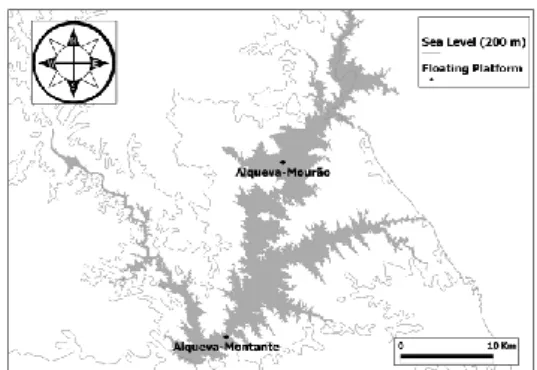
Figure 1 – Alqueva reservoir and floating platforms locations.
The Alqueva reservoir is located along 83 km of the main course of the Guadiana river and constitutes the largest artificial lake in the Iberian Peninsula (Figure 1). At the full storage level of 152 m, the reservoir has a total capacity of 4150 km3 and a surface area of 250 km2. Filling phase began in February 2002 and the reservoir is used for water storage and supply, irrigation and hydroelectric power generation. During the wet season, the water quality is controlled by inorganic contents with higher concentrations in the tributaries. In the dry season, the system is mainly controlled by the dissolved oxygen, pH and temperature.
Material and methods
This study was composed by a four months field campaign deployed in Alqueva reservoir shores and floating platforms (Figure 1). Measurements below water, air-water interface and above water were performed continuously and some of them punctual. Regarding continuously measurements, air-water interface momentum, heat and mass (H2O and CO2) fluxes are obtained with the new Campbell
Scientific’s IRGASON Integrated Open-Path CO2/H2O Gas Analyzer and 3D Sonic Anemometer. This system was mounted in a floating platform surrounded by a network of surface weather stations installed on the shores. See Figure 2 for details.
Figure 2 – Alqueva-Montante platform equipped with IRGASON instrument; Detail on sonic anemometer, gas analyser and acelerometer.
Together with the EC fluxes also radiative fluxes, both short and long wave, were measured in the platform in order to assess the radiative balance. Water temperature profiles were continuously recorded ate several depths allowing for water column heat storage calculations.
The EC method allows for a better assessment of the water-air interactions. This technique uses high frequency measurements, typically 20 Hz, and 30 minutes averaged fluxes. Depending on the equipment some corrections need to be done in order to have corrected fluxes. In this case, three corrections are necessary due to instrument surface heating/cooling: first the three dimensional coordinate rotations, which result in zero vertical and transverse mean wind speeds, are applied to the covariances; second the correction of density fluctuations for thermal expansion and water vapour dilution according, and third the sonic temperature is corrected for water vapour according Kaimal and Gaynor (1991). The corrected turbulent fluxes obtained are (in the following equations ̂ ̂ ̅̅̅̅̅̅ represents the rotated covariances between a and b): Momentum flux: ̂ ̅̅̅̅̅̅ ̂
Where is air density ;
(
) is density of dry air ; where
is the ratio of the molecular weight of dry air to water vapor and is the temperature corrected for water vapour: ( ) ; е is vapour pressure of water in air and p is absolute pressure. Sensible heat flux: ̅̅̅̅̅̅̅̂ ̂
Where is specific heat of air (1003.5 J Kg-1 K-1). Latent heat flux:
̅̅̅̅̅̅̅̅ (̂ ̂
̅̅̅̅
) ̂ ̂
̅̅̅̅̅̅̅̅
The second term for water vapour dilution and the third for thermal expansion (both correction of density fluctuations for water vapour), where is the molecular mass of air.
Carbon dioxide flux: ̅̅̅̅̅̅̅̅ (̂ ̂ ̅ ) ̂ ̂ ̅̅̅̅̅̅̅̅ ( ̅̅̅̅ ) ̅ ̅̅̅̅̅̅̅̅̂ ̂ Again, the second term for water vapour dilution and the third for thermal expansion (both correction of density fluctuations for water vapour).
After averaging some filters need to be applied to the 30 minutes fluxes. The fluxes are validated according the wind direction (only from the fetch), the footprint, the signal strength of the gas analyzer and the outliers. The fetch consider was between the angles 270º and 90º in order to avoid the contamination of platform to the measurements (See Figure 3). With this flag 35.2% of the measurements were discarded. The footprint analysis was made according Kljun et al. (2004), for 90% contribution (X90) and peak contributing (Xmax) distances:
( )
( )
Where is the standard deviation of vertical velocity fluctuations, [( ̅̅̅̅̅̅) ( ̅̅̅̅̅̅) ] is the friction velocity, is sensor height, and are parameters function of roughness length
(Z0). In this work Z0 was computed according Zilitinkevich (1991):
; ;
Where is air viscosity and
.
Calculation of atmospheric stability parameter ( ) was done for this field campaign using the Monin-Obukhov length (L):
̅ ̅̅̅̅̅̅̅
Where is the von Karman constant.
Punctual measurements of downwelling zenith hemispherical radiance (irradiance) were performed with a new apparatus developed following the version of Potes et al. (2013). The old version allows for attenuation coefficients calculations only from the inflexion point of downwelling radiance. Due to is small FOV (22º) and under small solar zenith angles this inflexion point varied from 0.25 to 0.5 m. Thus, the need to have measurements independent on solar zenith angle a new tip was developed to measure the hemispherical radiance (irradiance) allowing for attenuation coefficient calculations from the sub-surface level to 3 meters depth. See Figure 3 for details.
Figure 3 – Detail of optical receiver and multi-layer protecting frame of underwater device for measuring downwelling spectral irradiance; Measurements during ALEX2014 field campaign in Alqueva reservoir.
This version was also tested in a five-meter deep pool from the municipal swimming complex of Évora. After the test sessions, the apparatus was used to perform measurements in Alqueva reservoir in the summer of 2014 during ALEX2014 field campaign (Figure 3).
All the measurements campaigns were conducted under clear sky conditions. The length of the optical cable allows for measurements to a maximum depth of 3 m and the levels chosen for the profiles were: Surface, 0.01, 0.25, 0.50, 0.75, 1.00, 1.50, 2.00, 2.50 and 3.00 m. Before every profile measurement, the integration time of the spectroradiometer was optimized to ensure the best conditions of the lighting state. Also a dark current spectrum (which is an offset that varies with the temperature of the detector) was taken before every profile in order to correct the signal from temperature oscillations. We chose a sample average of ten spectra and three samples were taken per level. This choice was looking for equilibrium between a preferentially high number of spectra per level and a relative fast profile to keep similar atmospheric conditions.
Results
In Figure 4 is shown the X90, in meters. The average value of X90 is 105.9 m and for Xmax is 52.8 m, not shown here.
Figure 4 – Footprint length (X90) in meters from the fetch consider.
In Figure 5 is shown a scatter plot between footprint and atmospheric stability during the field campaign period, June to September 2014. It is clear visible the two regimes which are function of roughness length calculations (two equations for Z0 with friction velocity threshold). Lower friction velocities correspond to higher instability (lower z/L) and generate lower footprints.
Figure 5 – Scatter plot of footprint (X90) and stability (z/L) during
the period June-September 2014.
In Figure 6 is presented a plot of average daily variation of stability parameter (z/L) and CO2 flux for the period 22 to 26 July, an Intensive Observation Period (IOP) carried out during the four months campaign. During this period additional measurements were performed including the boundary layer characterization through radiosondes and passive remote sensing (not shown here). It is visible some correlation between stability and carbon dioxide flux. During night and morning greater instability agree with greater carbon uptake by the lake, on the other hand during afternoon and under stability conditions a small release of carbon is notice from the lake to the atmosphere.
Figure 6 – Mean daily cycle of instability (z/L) and CO2 flux
during 22 to 26 July, an Intensive Observation Period (IOP).
Results from the mean daily cycle of carbon dioxide flux for the four months period (Figure 8) show the same behaviour as in IOP (Figure 6) but always with negative fluxes. This means that lake acts has a sink for carbon dioxide. Lower values were found during night and early morning and higher values during afternoon (near zero). Nevertheless, this result represents only four months of the year (June to September) and further long-term studies are necessary to fully characterize the carbon cycle in Alqueva reservoir.
Figure 8 – Mean daily cycle of CO2 flux during the period
June-September 2014.
Mean daily cycle of sensible heat flux and temperature difference between air (2-meters) and water skin is shown in Figure 9. Is clear visible that for positive values of sensible heat flux the temperature difference is negative (except for 13:00) and vice-versa.
Figure 9 – Mean daily cycle of sensible heat flux and temperature difference between air (2-meters) and water skin, during the period June-September 2014.
This means, during afternoon when air temperature is higher than water skin temperature there is conditions for development of a lake breeze allowing the subsidence of upper drier air leading to an increase of latent heat flux (Figure 10) and forcing a negative sensible heat flux. There is also in this period that stability conditions were found (Figure 6).
Figure 10 – Mean daily cycle of latent heat flux and water vapour, during the period June-September 2014.
Using the latent (LE) and the sensible (H) heat fluxes, the net radiation (Rn), and computing the water column heat storage ( ) the energy balance at the surface can be obtained, assuming horizontal homogeneity and neglecting the heat fluxes due to precipitation, runoff and bottom sediments, through the equation below:
With ∑ , where is
specific heat of water (4192 J Kg-1 K-1).
After some numerical experiments we found that, at an hourly basis, better results for were obtained taking into account only the first 4 meters. The average diurnal cycle of the four terms of (June to September) are shown in the Figure 11. According to this plot the mean available energy in terms of absolute residual ( ) is 86.1 W m-2.
Figure 11 – Mean daily cycle of net radiation (Rn), water column heat storage (∆Q), latent heat flux (LE) and sensible heat flux (H), during the period June-September 2014.
Measurements of downwelling irradiance were performed in a clear water pool of Evora municipal
swimming complex before the field campaign. Then periodic measurements were performed at Alqueva reservoir during the field campaign. Figure 4 shows two profiles of downwelling zenith irradiance performed at the pool on 14 of July 2014 and at Alqueva reservoir on 27 August 2014. These two profiles present similar spectral behaviour on the region 700-900 nm with a fast decay on the irradiance but different behaviour on the rest. In the pool the irradiance penetrates deeper on the range 400-500 nm while in Alqueva on 500-600 nm. At 3 meters depth in the pool we have more than 50% of surface irradiance between 400 and 600 nm. At the same depth in Alqueva we have 1 to 10% between 500-700 nm. It means that in Alqueva the euphotic depth is reach (for almost the wavelengths) within the 3 meters profile.
Figure 12 – Profiles of underwater downwelling spectral irradiance in municipal swimming complex of Évora (left) and in Alqueva reservoir. Profiles are in percentage of surface irradiance.
The average attenuation coefficient for the range 400-700 nm was computed, which is frequently called PAR (Photosynthetically Active Radiation) region. In Table I are represented the PAR attenuation coefficient of the most significant profiles obtained in the campaign. This spectral region concentrates about half of the solar radiation, thus the radiance is able to penetrate deeper in PAR region than outside of it (Figure 12). Therefore, most of the water quality studies over lakes and lagoons focus on PAR region (Potes et al., 2011).
Tabela I – Measurements details. Turbidity and PAR attenuation coefficient for the layer 0-3 m.
Date Local PAR Attenuation Coefficient (m-1) 14/07/2014 Pool 0.163 27/08/2014 Alqueva - Montante 1.074 27/08/2014 Alqueva - Mourão 1.102 25/09/2014 Alqueva - Montante 1.039 25/09/2014 Alqueva - Mourão 1.434
Conclusion
Measurements of energy and mass (H2O and CO2) fluxes were continuously obtained from June to September 2014 from a floating platform in Alqueva reservoir, southeast of Portugal. During this period the temperature gradient between the atmosphere and reservoir presents two opposite behaviours during the daily cycle. It is observed a positive gradient during afternoon, in this way, a negative sensible heat flux is noticed in afternoon and a lake breeze is developed locally allowing the subsidence of upper layers dry air to reach the surface in the centre of the reservoir. Consequently, stable atmospheric conditions are noticed in the afternoon and unstable in the rest of the day. Latent heat is higher also in the afternoon with an average maximum around 20UTC. The average daily cycle of CO2 flux presents negative values during all day, with a maximum uptake by the reservoir in the evening, the period of maxima CO2 concentration in the atmosphere due to plants respiration. The energy balance was estimated for the surface of the reservoir. Heat storage calculations (ΔQ) plays an important role and further calculations need to be done for better accuracy. Nevertheless, the reservoir is accumulating energy in this four summer months. A new apparatus was developed to be coupled with a portable spectroradiometer, allowing for spectral downwelling irradiance measurements in underwater environment and to obtain estimates of the light attenuation coefficient in water. It ensures spectral downwelling irradiance measurements with a FOV of 180, in the range 325-1075 nm, with a moderately high spectral resolution of 1 to 3 nm from the visible to the near infrared. The exponential decrease of irradiance with depth was verified, allowing the calculation of the attenuation coefficient through the exponential law. Thus, the attenuation coefficient retrieved in this work is assumed to be the diffuse attenuation coefficient, which is a property of the medium independent of the illuminating light field (inherent optical property). The comparison of the PAR attenuation coefficient from the different field campaigns confirms that an increase in water turbidity leads to an increase in PAR attenuation coefficient. This coefficient is a key parameter for lakes models, which are intended to be coupled to weather forecast models (Balsamo et al., 2012). A future aim of this work is to collect attenuation coefficient values of worldwide lakes, dams and reservoirs in order to develop a robust satellite-based algorithm to enlarge the attenuation coefficient network for the major lakes on Earth.
Acknowledgements
The authors acknowledge the funding provided by ICT, under contract with FCT (the Portuguese Science and Technology Foundation). Experiments were accomplished during the field campaign
funded by FCT and FEDER-COMPETE: ALEX 2014 (EXPL/GEO-MET/1422/2013) FCOMP-01-0124-FEDER-041840. The work was supported by FCT PostDoc grant SFRH/BPD/97408/2013.
References
Balsamo, G., Salgado, R., Dutra, E., Boussetta, S., Stockdale, T., and Potes, M. 2012. On the contribution of lakes in predicting near-surface temperature in a global weather forecasting model. Tellus, 64A, 15829.
Kaimal, J.C. and Gaynor, J.E., 1991. Another look at sonic thermometry. Boundary Layer Meteorology, 56: 401-410.
Kljun, N., P. Calanca, M.W. Rotach, H.P. Schmid: 2004, 'A Simple Parameterisation for Flux Footprint Predictions', Boundary-Layer Meteorology, 112, 503-523.
Mironov, D. V., Heise, E., Kourzeneva, E., Ritter, B., Schneider, N. and Terzhevik, A. 2010. Implementation of the lake parameterisation scheme FLake into the numerical weather prediction model COSMO. Boreal Env. Res. 15, 218-230.
Nordbo, A., S. Launiainen, I. Mammarella, M. Lepparanta, J. Huotari, A. Ojala, and T. Vesala, 2011. Long-term energy flux measurements and energy balance over a small boreal lake using eddy covariance technique. J. Geophys. Res., 116, D02119, doi:10.1029/2010jd014542.
Potes, M., Costa, M. J., Silva, J. C. B., Silva, A. M., and Morais, M.2011. Remote sensing of water quality parameters over Alqueva reservoir in the south of Portugal. Int. J. Remote Sens. 32:12, 3373-3388.
Potes, M., Costa, M. J., Salgado, R. 2012. Satellite remote sensing of water turbidity in Alqueva reservoir and implications on lake modeling. Hydrol. Earth Syst. Sci. 16, 1623-1633.
Potes, M., Costa, M. J., Salgado, R., Bortoli, D., Serafim, A. and Le Moigne, P. 2013. Spectral measurements of underwater downwelling radiance of inland water bodies. Tellus-A, 65, 20774.
Salgado, R. and Le Moigne, P. 2010. Coupling of the FLake model to the Surfex externalized surface model, Boreal Environ. Res. 15, 231-244.
Zilitinkevich, S.S., (Ed.) 1991. Modeling Air-Lake Interaction. Physical Background (authors: E.E. Ferdorovich, S.D. Golosov, K.D. Kreiman, D.V. Mironov, M.V. Shabalova, A.Yu. Terzhevik and S.S. Zilitinkevich), Springer Verlag, Berlin, 130 pp.