1 Work Project, presented as part of requirements for the Award of a Master Degree in Economics from NOVA – School of Business and Economics (Portugal) with Double Degree
Partnership with INSPER (Brazil)
Bolsa Família Program Impact on the composition of Brazilians families’ expenditures
Lauro Américo dos Santos
A project carried out on the Master in Economics Program, under the supervision of: Priscila Ribeiro (INSPER)
Susana Peralta (NOVA)
2 ABSTRACT
Bolsa Família Program Impact on the composition of Brazilians families’ expenditures
Conditional Cash Transfers Programs are being popular in Latin America as a way to deal with poverty. This work focusses on analyzing how Bolsa Família recipients allocate their transfers and if they are spending efficiently to overcoming poverty. We used Propensity Score Matching under the microdata available on the Household Budget Survey 2008-2009 published by IBGE. The main results of this work are an average increase of 10% on food expenditures and an increase of 9.4%, on average, for total expenditures in the 40% poorest quantile, addressing poverty alleviation and ensuring better social conditions.
3 1Introduction
A simple way of defining poverty is as a condition in which household’s income is lower than it is necessary for ensuring their basic living standards. It is most often measured in monetary terms, captured by level of incomes or consumption per capita or per household. One of the most usual thresholds to determine households living in extreme poverty situations is the World Bank US$ 1.90 income per day limit and, in 2013, it was estimated that 767 millions of people were living under this limit, with great reduction in the last 20 years. The World Bank (2016) lists a series of policies implemented throughout several countries considered as effective for this extreme poverty reduction, i.e., investments in rural infrastructure, universal access to health care and good-quality education, taxation and conditional cash transfers (CCT).
In Brazil, the 1988 Constitution adopted after 20 years of dictatorship is a marker for social assistance programs by guaranteeing basic social rights such as free public education, health care and pensions. However, the social security system created was based on formal workers and policies to address poverty focused on old age households and on disability, failing to address child poverty. Furthermore, economic distress that generated high unemployment rates limited the programs’ efficiency (The World Bank, 2016, Barrientos et al, 2016).
4 One of the largest CCT programs in the world is the Brazilian Bolsa Família, implemented by the end of the 90’s and in the beginning of the 00’s consolidating five different programs throughout the country: Bolsa Escola, Bolsa Alimentação, Cartão Alimentação, Auxílio Gás
and PETI. The Federal Government, with higher financial and operational capacity, scaled them nationwide, naming it Bolsa Família, standardizing eligibility criteria and benefit levels. According to MDS (2017), households with a per capita monthly income up to R$ 85 (US$ 43) are eligible for receiving transfers, while households with a per capita income within a R$ 85 (US$ 43) and R$ 170 (US$ 85) range are only eligible due a specific family structure and with conditions for receiving transfers (expenses in Reais were converted into US dollars using a purchasing power parity bases, PPP 2016: US$ 1 = R$ 1.99). Currently, 25% of the Brazilian population is BF recipient.
5 The rest of this work is organized as follows. Section 2 reviews the literature about CCT programs and Bolsa Família Program. Section 3 presents the database used for this work and the statistical method that I used in this work. Section 4 presents results and Section 5 summarizes main conclusions.
2Conditional Cash Transfer Overview and Bolsa Família Program
In this section, I provide an overview about Conditional Cash Transfers (CCT) programs and the Bolsa Família Program (BFP). The first subsection presents a literature review about these kinds of programs around the world and their history. The second subsection present a BFP evaluation, its requirements and summarizes some studies already presented about it.
2.1 Conditional Cash Transfers
CCT programs aim to alleviate current poverty while at the same time that ensuring lower future poverty by augmenting human capital levels of children, thus increasing their lifetime earnings potential. Recipient households commit to conditions for receiving benefits, i.e., children’s school attendance and family visits to health clinics.
These innovative programs began with Mexican Oportunidades and Brazilian Bolsa Família in the end of the 90’s, as a second-generation type of program for addressing poverty in Latin America.
6 In Brazil, Bolsa Família was created in 1996, covering 14 million families and is similar to
Oportunidades in terms of coverage and importance. However, it is softer on conditions and has greater emphasis on income redistribution rather than human capital formation. Bolsa Família did not explicitly incorporate impact evaluations in its design and, as a result, much less is known about impacts on consumption, poverty, health, nutrition and education (Fiszbein, 2009, MDS, 2017).
Chile Solidário was created in 2002, focusing on extreme poverty families and reaches 5% of Chile’s population. Its design is distinct to other CCT programs, since households work with social workers to understand actions for overcoming extreme poverty, committing to action plans that become the conditions for receiving the benefit. The cash transfer itself is intended to be a motivation for families to make use of the social workers’ services for a limited time (Fiszbein, 2009).
Many other CCT programs have spread throughout Latin America and the Caribbean, reaching, in 2010, almost 130 million recipients, representing a quarter of the region’s population, distributed in 18 countries (Stampini and Tornarolli, 2012).
7 2.2 Bolsa Família Program
Although Bolsa Família is considered as the largest CCT in Latin America,it only conditions cash transfer for households within a R$ 85 (US$ 43) and R$ 170 (US$ 85) per capita income/month range. For them, the household’s benefits level depends on the family structure as described in Table 1. Households that are in extreme poverty, with less than R$ 85 per capita income/month do not have to comply with conditions to receive benefits. Besides that, benefits are calculated on a case-by-case basis, so they can receive R$ 85 per capita income. Expenses in Reais were converted into US dollars using a purchasing power parity bases, PPP 2016: US$ 1 = R$ 1.99 (Soars et al., 2009) (MDS, 2017).
The entry of households into the Bolsa Família Program is done through registration in the
Cadastro Único system, created in the unification process of the previous benefits that aims to centralize the Brazilian low-income families’ socioeconomic records. Until May 2017, according to the Social Development Ministry (MDS, 2017), more than 27.5 million families had been registered, corresponding to almost 80 million people. On these families, 12.7 million have a per capita income up to R$ 85 and 3.8 million between R$ 85 and R$ 170.
8 Table 1 Bolsa Família Program variable benefits description
Benefits Cash Transfer Conditioning
Households with monthly per capita income lower than R$ 85,00 (US$ 43) Overcoming poverty
benefit
Calculated on a case-by-case basis to ensure at least R$ 85
income per capita/month.
Not needed.
Households with monthly per capita income within R$ 85,00 – R$ 170,00 (US$ 43 – US$ 85)
Variable by children
from 0 to 15 years old R$ 39
School attendance of 85% is required.
Variable by Pregnant Benefit
R$ 39 for 9 months
Pregnancy identified and monitored by health area Breastfeeding
Variable Benefit
R$ 39 for 6 months
Children must have data included in Cadastro Único
until sixtieth month of life. Variable by Teenagers
from 16 to 17 years old
R$ 46 School attendance of 75% is required.
Source: MDS 2017.
9
al. (2010), there is a volatility income effect to households at the poverty line that could generate social vulnerability and incentives for the program to continue benefiting households slightly above the limit, as it may occur that withdrawing the benefits, those families could return to poverty and should suffer severe effects on the lag of children in schools, for instance.
According to MDS (2017), conditionality is periodically verified and households that fail to prove children’s regular school attendance and immunization schedule are warned that benefits could be suspended. According to Senna et al. (2016), 90% of the conditionalities related to education are followed with small variations between municipalities. 75% of health conditionalities, however, are monitored, with strong growth since 2005.
MDS (2017) reports that households are advised to register changes in address, birth or death of family members, increase or decrease in income, among other events as soon as they occur. The main reason that leads families to be disqualified from the program is lack of registration updates or increase in households’ income, making them no longer a target by the program. Benefit cancellations due to noncompliance conditions are used only as a last resort, since the program’s objective is to reinforce the access of families in need of social rights.
Oliveira et al. (2007), comparing recipients and non-recipients with similar income, present positive results regarding children’s school enrollment, reducing classes absence and dropout probabilities. The authors also show, however, that children that are Bolsa Família recipients are more likely to fail than those who are not, possibly because students who have been out of classes have greater difficulties in following lessons comparing to those who have always attended to school (Soares et al., 2010). Jones (2016) reaches similar conclusion, but questions whether the human capital development aspect of the program will be achieved as it is not clear what level of quality and preparation Brazilian schools are offering these students. Barrientos
10 depending on gender, with municipalities with less girls attending to school showing stronger attendance effects, as an equalizing effect.
Regarding health-related impacts, Soares et al. (2010) concludes that the program has not yet impacted infant immunization rates, despite of its conditionalities. There is no data to conclude whether the number of medical appointments has increased. This effect could be related to the lack of essential health services in municipalities.
Few authors, however, focus their studies on recipient household’s consumption expenditure. Resende and Oliveira (2008) analyzed the effects of the Bolsa Escola in household spending, comparing consumption patterns between recipient and non-recipient households in the
Pesquisa de Orçamentos Familiares (POF – Household Budget Survey) 2002-2003. The authors use a matching algorithm based on households’ observable characteristics to create a control group, allowing them to obtain a causal estimate of the program. Resende and Oliveira (2008) were able to analyze the program effect on food, housing, clothing, education and other expenses, concluding that recipient families are more likely to improve family’s diet, both in quantity and diversification, as well as obtaining items related to children’s education, hygiene and health. Consumption of items such as alcoholic beverages, cigarettes and miscellaneous expenses are diminished.
11 3Data and Methodology
In this section I describe the databases and statistical models used in this work.
3.1 Database
This work is based on the microdata from the Household Budget Survey (POF) 2008-2009, published by IBGE. POF is a representative household-based survey, in which household, or consumption unit, is defined as one or more residents who share the same source of food or living expenses.
According to IBGE (2011), the POF’s aim is to publish information on expenses, income and wealth evolution of Brazilians families, providing data for studies about domestic budgets and consumers’ expenses structure, that are used to measure Brazil’s official inflation index, IPCA. POF also provides socioeconomic information such as occupation, types of households, sanitary disposal, water supply and energy, as well as food consumption habits. The survey is conducted every five years, although the most recent research collection started only in 2017, to be available in 2019.
The sample is representative at national level, at large regions level (North, Northeast, Southeast, South and Center-West) and at urban and rural regions level. Detail by federation unit would be representative for the total and urban areas, while details by metropolitan regions and unit federation capitals correspond only to urban areas (IBGE, 2011).
12 As part of the household income description, POF 2008-2009 distinguishes between monetary and non-monetary income. The first group of income corresponds to income from work (gross remuneration from work as an employee, employer and self-employed), as well as transfers from public and private pensions, pensions and federal social programs, such as Bolsa Família, BPC assistance and Child Labor Eradication Program (PETI). It is possible to clearly identify which households receive those transfers and their social conditions, eating habits and consumption patterns.
According to IBGE (2011), for POF 2008-2009 edition, Brazil was divided into 4,696 sectors, corresponding to 55,970 households and 56,091 consumption units. Considering expansion factors provided by IGBE, this research sample represents 57,816,604 households with 190,519,297 persons.
3.2 Propensity Score Matching Estimator
The main challenge in empirical policy evaluation is how to overcome the bias that stems from participant’s selection into treatment. Since Bolsa Família concentrates its transfers to poor households in a country with high social inequalities, a simple average expenditure comparison between the program’s recipients and the rest of the population is not an acceptable approach to evaluate the program’s expenditure effect on the poor.
13 To be more precise, let Di be an indicator variable of whether or not household i is a recipient of Bolsa Família:
!" =
1, &' ℎ*+,-ℎ*./ &, 0-1&2&-34 0,
*4ℎ-06&,-Setting as 78" the outcome variable for household i if it is a BF’ recipient and 79" otherwise, the average treatment effect on the treated (ATT) is given by
Equation 1 :;; = < 78"− 79" !" = 1 = < 78" !" = 1 − < 79" !" = 1
Since < 79" !" = 1 is impossible to observe, since a given household cannot be simultaneously recipient and non-recipient, we need to rely on the outcome of non-recipient households < 79" !" = 0 as an approximation. However, we need to ensure that the outcomes can be considered equal, i.e., < 79" !" = 1 = < 79" !" = 0 .
If it were possible to identify non-participant households that are similar to treatment group through a vector (X) consisting on observable characteristics and other characteristics that could potentially influence treatment selection, we should have
Equation 2 < 78"− 79" !" = 1, > = < 78" !" = 1, > − < 79" !" = 0, >
By constructing an appropriate control group, similar to the treatment one, except in the recipient (or treatment) status, we can assume that the outcomes are independent to the distribution of which group household i would be (control or treatment). This way, we can conclude that (79"78" ⊥ !") according to the Conditional Independence Hypothesis (CIA), leading us to determine that
Equation 3 < 79" >", !" = 1 = < 79" >", !" = 0
14 identification when calculating the probability of a non-recipient household presenting similarity to treatment group given the characteristics vector X.
Rosenbaum and Robin (1983) demonstration allows determining that:
Equation 4 < 78"− 79" !" = 1, B(>) = < 78" !" = 1, B(>) − < 79" !" = 0, B(>)
It is important to emphasize that two hypotheses are mandatory for an unbiased evaluation: independent households’ selection from outcomes and common support between treatment and control groups, i.e., for each recipient household, there’s at least one household that has similar probability of being a program participant, considering the characteristics vector X. (Rosenbaum and Rubin, 1983) (Cerulli, 2015).
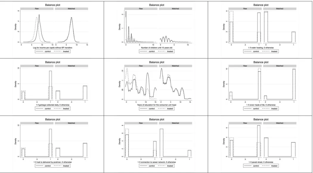
There are several algorithms for matching control and treatment groups, namely, nearest neighbor (NN), which can be with or without replacement; caliper and radius; stratification and intervals; among others (Caliendo and Kopeining, 2008). Sensitivity Analysis is an important step as described by Garrido et al. (2014) suggesting balancing analysis between treatment and control groups by comparing standardized differences, distributions graphs and variance ratios, especially for confounders hypothesized to be strongly related to the outcome. In this work, we calculated propensity score through a probit model considering the characteristics vector X and used this as an input for a propensity score estimator. In this method, each treated household is paired with one household in control group who has the nearest propensity score. I made balancing analysis through standardized differences, balance graphs and propensity score box plots.
3.3 Data and variables description
15 households. Excluding the income of the program, these families receive monthly, on average, R$ 167.44 per capita.
According to MDS (2017), by the time of the survey, Bolsa Família target population were families within poverty range (per capita income per month of R$ 77.01 to R$ 154, as long these families include children, teenagers, pregnant women and breastfeeding women) and extreme poverty range (per capita income per month below R$ 77, considering any family structure).
Table 2 Dependent variables description
Monetary expenditures Description
Food Food acquisition for both inside and outside consumption.
Clothing Men’s, women’s, children’s clothes, footwear, jewelry, fabrics and haberdashery.
Education Regular courses, higher education, textbooks, school articles and other related expenses.
Housing, Transportation,
Hygiene and Health Care
Housing expenditures account for rent, services as telephone, water,
gas, electricity, house maintenance, furniture and repairs.
Transportation expenditures account for urban transportation, vehicles
acquisition and maintenance, sporadic trips among other related items.
Hygiene expenditures account for perfumes, hair products, soap and
other instruments and products for personal use.
Health Care expenditures account for medicines, health plans, medical
and dental treatments, surgeries, hospitalizations, among other related
expenses.
Other items
Toys, games, cell phones and accessories, non-didactic books and
magazines, cigarettes and tobacco, personal services i.e., hairdressing,
manicure and pedicure services; taxes, labor contributions, banking
services, pensions, allowances and donations.
Total Expenditures Sum of the expenditures above.
Source: Household Budget Survey – POF 2008-2009/IBGE. Self-Elaboration.
16 Average expenses decomposition for BF recipients is available in Figure 1. Food expenditures account for 33% of total expenses budget as the largest household’s expenditure, followed by Housing (23%), Transportation (15%), Clothing (7%), Health Care (5%) and Hygiene and Personal Items (4%).
Figure 1 Average expenditures decomposition for BF recipients.
Source: Household Budget Survey – POF 2008-2009/IBGE. Self-Elaboration.
To meet propensity score matching model requirements, I used observable households’ characteristics as independent variables considering the Bolsa Família selection model itself and sample distributions of other observable characteristics among control and treatment group. Examples of independent variables are income per capita without the transfers, urban or rural location indicator, a set of variables indicating the materials in which the domiciles were built and what kind of public services are available. Information about the head of the consumer units and family structure was also considered.
The next session displays the results of the estimated models. Food
33%
Clothing 7% Education
2% Housing,
Transportation, Hygiene and Health
Care 47%
Other items 11%
17 4Results
Independent variables descriptive analysis for raw data, before any match was been done is available in Table 3. Since Bolsa Família has two target population range, I analyzed the program effects for the 40% and 20% poorest quantiles as well.
The 20% poorest quantile has an average income per capita without BF transfers of R$ 93.05 for total subsample and R$ 79.88 for BF’s recipients. This quantile recipients correspond to 48.7% of total subsample. We can approximate this quantile to the BF’s extreme poverty range (below R$ 77 per capita income/month).
The 40% poorest quantile has an average income per capita without any BF transfer of R$ 165.55 for total subsample and R$ 121.46 for BF’s recipients. This quantile recipients represent 35.9% of total subsample and corresponds to 86.9% from all recipients in the survey. It is important to mention that restricting the number of observations can affect the quality of the estimates, specially for the 20% poorest quantile.
Propensity scores matching models for all expenditures and subsamples are based on the nearest neighbor with replacement technique as an attempt to overcome this issue.
Infrastructure, social and health conditions in which BF’s households are located are more vulnerable, with a lower rate of garbage collection, piped water, street paving and connection to sewer networks; naturally, this becomes even lower when we concentrate on the 40% and 20% poorest quantiles. BF’s recipients have also shown a higher number of children and less years of education for the consumer units’ head.
18 Table 3 Independent variables descriptive statistics for raw data
19
Table 4 Propensity score probit regression for total expenditures model
Total 40% Poorest 20% Poorest
Coef. (Std. Err.) 95% CI Coef. (Std. Err.) 95% CI Coef. (Std. Err.) 95% CI Households data
Located at urban area 0.03 (0.0269) [-0.02; 0.09] 0.00 (0.0315) [-0.06; 0.06] -0.01 (0.0415) [-0.09; 0.08] External wall made from
masonry 0.12* (0.0227) [0.07; 0.16] 0.14* (0.0264) [0.09; 0.19] 0.15* (0.0343) [0.08; 0.21]
Cover made of tile 0.13* (0.0249) [0.08; 0.18] 0.15* (0.0306) [0.09; 0.21] 0.20* (0.0417) [0.12; 0.29]
Floors made of cement 0.20* (0.0169) [0.17; 0.24] 0.18* (0.0203) [0.14; 0.22] 0.16* (0.0280) [0.10; 0.21]
Existence of piped water -0.01 (0.0251) [-0.06; 0.04] 0.00 (0.0287) [-0.06; 0.06] 0.02 (0.0362) [-0.05; 0.10] Connection to sewer
network -0.06* (0.0209) [-0.10; -0.02] -0.07* (0.0262) [-0.12; -0.02] -0.09** (0.0375) [-0.16; -0.01]
Paved street -0.02 (0.0198) [-0.06; 0.02] 0.00 (0.0237) [-0.05; 0.04] 0.00 (0.0323) [-0.06; 0.06] Mail is delivered by
postman -0.05*** (0.0259) [-0.10; 0.00] -0.03 (0.0304) [-0.09; 0.03] -0.08** (0.0404) [-0.16; -0.01]
Garbage collected daily -0.06** (0.0235) [-0.10; -0.01] -0.10* (0.0276) [-0.15; -0.05] -0.11* (0.0366) [-0.19; -0.04]
Water heating -0.36* (0.0181) [-0.39; -0.32] -0.36* (0.0223) [-0.41; -0.32] -0.37* (0.0318) [-0.43; -0.31] Residents data
Income per capita without BF transfers (R$/month) -0.45* (0.0093) [-0.47; -0.44] -0.32* (0.0120) [-0.34; -0.29] -0.25* (0.0161) [-0.28; -0.22]
Number of children until 15 years old
0.30* (0.0065) [0.29; 0.31] 0.23* (0.0072) [0.22; 0.25] 0.21* (0.0089) [0.19; 0.22] Years of education for
the consumer unit head
-0.03* (0.0021) [-0.03; -0.03] -0.04* (0.0027) [-0.04; -0.03] -0.04* (0.0038) [-0.05; -0.03] Checking account for
consumer unit head
-0.21* (0.0340) [-0.27; -0.14] -0.24* (0.0500) [-0.34; -0.15] -0.33* (0.0877) [-0.50; -0.16] Number of
Observations 55,350 21,884 10,760
Pseudo R2 0.32 0.15 0.11
Source: Author’s computation using data from the Household Budget Survey – POF 2008-2009/IBGE. Significance Level: (* 1%) (** 5%) (*** 10%)
Propensity score matching models’ results are available in Table 5. I compared three models in
this work to analyze their robustness and respective Average Treatment Effect on the Treated
(ATT) through subsamples. Robust standard errors are presented according to Abadie and
Imbens (2016) model.
As propensity score matching model requires that there is a common support region between
20 with this requirement. As balance test for all covariates in the three models, average
standardized differences for matched observations is shown in Table 6 and variance ratios for
matched observation in shown in Table 7. Covariates balancing graphs are also available in the
Appendix section.
Figure 2 Total expenditures common support for total, 40% and 20% poorest subsamples
Source: Author’s computation using data from the Household Budget Survey – POF 2008-2009/IBGE.
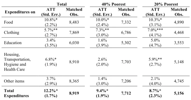
Food expenses raised, on average, by 10.8%, 10.0% and 10.3% for the entire sample, 40% and
20% poorest subsamples, respectively. The rise of expenses on food equates to results found by
Resende and Oliveira (2008) when analyzing the effects of Bolsa Escola transfers on
households’ budget expenditures using POF 2002-2003 microdata.
Clothing expenditures raised, on average, by 5.7% for total households and 7.3% for 40%
21 Housing, Transportation, Hygiene and Health Care expenses are considered as a single expense
account, to overcome issues of mismeasurement in individual terms. On average, this group
expenditure raised by 68% for total sample and by 5.9% to 20% poorest subsample.
Although education expenditures are positive, they are not statistically significant for any strata.
This category, however, was not added to another one since this is an important aspect of Bolsa Família Program. The higher standard errors for this expenditure and fewer matched
observations seems to compromise these models’ statistical significance.
Other items effects results are not statistically significant for any strata. Considering
households’ total consumption, Bolsa Família seems to rise, on average, 8.7% to 12.2%,
depending on which strata is analyzed.
Table 5 Average treatment effect on the treated (ATT) for listed expenditures
Total 40% Poorest 20% Poorest
Expenditures on ATT (Std. Err.) Matched Obs. ATT (Std. Err.) Matched Obs. ATT (Std. Err.) Matched Obs.
Food 10.8%*
(2.2%) 8,483
10.0%*
(2.4%) 7,332
10.3%*
(3.1%) 4,890
Clothing 5.7%**
(2.7%) 7,869
7.3%**
(3.0%) 6,786
7.0%***
(4.1%) 4,468
Education 3.4%
(3.5%) 6,030
1.6%
(3.9%) 5,302
5.0%
(4.7%) 3,553
Housing, Transportation, Hygiene and Health Care
6.8%*
(1.9%) 8,910
2.6%
(2.0%) 7,703
5.9%**
(2.7%) 5,148
Other items 3.7%
(2.9%) 8,365
1.4%
(3.0%) 7,206
2.1%
(4.0%) 4,745
Total
Expenditures
12.2%*
(1.7%) 8,919
9.4%*
(1.9%) 7,712
8.7%*
(2.3%) 5,156
Source: Author’s computation using data from the Household Budget Survey – POF 2008-2009/IBGE. ATT: Average treatment effect on the treated.
22
Table 6 Standardized differences for matched households
23
Table 7 Variance Ratios for matched households
24
5Conclusions
Conditional cash transfers programs, as Bolsa Família, are known as a great way of reducing
poverty by transferring income directly to head of families which can decide by themselves
how they spend the benefit. On the other hand, some recipients must ensure school attendance
for children and teenagers and health checkup in order to continue receiving transfers. This
way, the Federal Government helps to alleviate poverty while ensuring human capital formation
so that in the next generation these families can leave social vulnerability situations.
Since Bolsa Família recipients have full autonomy to spend their benefit, this work aimed to
identify through their budget structure, what effects these benefits cause or, in other words, how
they spend those payments. Using microdata from the Household Budget Survey POF
2008-2009 published by IGBE with Propensity Score Matching Estimators, Bolsa Família recipients
were identified as treatment group and compared to the rest of the sample through observed
characteristics that identified which families were non-recipients, but were eligible to be.
Sensitivity analysis were also made to ensure that models held important assumption, as
conditional Independence Hypothesis and common support through treatment and control
groups for all propensity scores calculated.
This work main findings were an average increase of 7.6% to 10.3% on total expenditures,
depending on which model is being analyzed, total (10.3%), 40% poorest (7.6%) or 20%
poorest households (7.9%). Food expenditures rise by 10.5% to 11.4% for BF recipients, on
average, followed by clothing expenditures rising by 5.4% to 5.8%, on average. Although
education expenses did not show statistical significance, housing, transportation, hygiene and
health care group of expenses rise by, on average, 9.6% for total recipients model.
When analyzing these results with the BF aim, it seems that those benefits are being spent
25 consumption. Food expenditures increase, for instance, ensure a better diet for households, in
particular children, allowing them to receive more nutrients and have better conditions to study
as an incentive for human capital formation.
This work contributes to increase the Bolsa Família Program understanding of how recipient
households manage resource allocation of their benefit.
6References
Abadie, Alberto; Imbens, Guido. 2016. “Matching on the estimated propensity score”.
Econometrica. 84(2): 781-807.
Adato, Michelle; Hoddinott, John. 2007. “Conditional Cash Transfer Programs: A “Magic Bullet” for reducing Poverty?.” 2020 Focus Brief on the World’s Poor and Hungry People. Washington, DC: IFPRI.
Barrientos, Armando et al. 2016. “Heterogeneity in Bolsa Família outcomes.” The Quarterly
Review of Economics and Finance, 62: 33–40.
Caliendo, Marco; Kopeinig, Sabine. 2008. “Some Practical Guidance for the Implementation of Propensity Score Matching.” Journal of Economic Surveys. 22(1): 31-72.
Cameron, A. Colin; Trivedi, Prakin K. 2005. Microeconometrics: Methods and Applications.
New York: Cambridge University Press.
Cerulli, Giovanni. 2015. Econometric Evaluation of Socio-Economic Programs Theory and
Applications. Springer.
Fiszbein, Ariel et al. 2009. Conditional Cash Transfers:Reducing Present and Future Poverty. Washington: The World Bank.
Garrido, Melissa M. et al. 2014. “Methods for Constructing and Assessing Propensity Scores.”
HSR: Health Services Research. 49(5): 1701-1720.
Instituto Brasileiro de Geografia e Estatística (IBGE). 2011. Pesquisa de Orçamento
Familiar (POF): 2008-2009: Análise do consumo alimentar pessoal no Brasil. Rio de Janeiro:
26 Jones, Hayley. 2016. “More Education, Better Jobs? A Critical Review of CCTs and Brazil’s Bolsa Família Programme for Long-Term Poverty Reduction.” Social Policy & Society. 15:3: 465-478.
Martins, Ana Paula; Monteiro, Carlos. 2016. “Impact of the Bolsa Família program on food availability of low-income Brazilian families: a quasi-experimental study”. BMC Public
Health. 16:827
MDS, Ministério do Desenvolvimento Social. 2017. Accessed June 14. http://mds.gov.br/assuntos/bolsa-familia/o-que-e/beneficios.
Oliveira, Ana Maria H. C. et al. 2007. “First Results of a Preliminary Evaluation of the Bolsa Família Program.” In: Evaluation of MDS Policies and Programs – Results Volume 2 – Bolsa
Família Program and Social Assistance, ed. Jeni Vaitsman; Rômulo Paes-Sousa, 19-64,
Brasília: Cromos Editora e Indústria Gráfica Ltda.
Resende, Anne C. C.; Oliveira, Ana M. H. C. de. 2008. “Avaliando Resultados de um Programa de Transferência de Renda: o Impacto do Bolsa-Escola sobre os Gastos das Famílias Brasileiras.” EST. ECON. 38(2): 235-265.
Rosembaum, Paul R.; Rubin, Donald B. 1983. “The Central Role of the Propensity Score in Observational Studies for Causal Effects.” Biometrika. 70(1): 41-55.
Senna, Mônica de C. M.; Brandão, André A.; Dalt, Salete da. 2016. “Programa Bolsa Família e o acompanhamento das condicionalidades na área de saúde.” Serviço Social &
Sociedade. 1: 148-166.
Soares, Sergei et al. 2009. “Conditional Cash Transfers in Brazil, Chile and Mexico: Impacts upon Inequality.” Estudios Económicos. Extraordinário: 207-224.
Soares, Fábio V. et al. 2010. “Evaluating the Impact of Brazil's Bolsa Família: Cash Transfer Programs in Comparative Perspective.” Latin American Research Review. 45(2): 173-190.
Sperandio, Naiara et al. 2017. “Impacto do Programa Bolsa Família no Consumo de Alimentos: Estudo Comparativo das Regiões Sudeste e Nordeste do Brasil.” Ciência & Saúde
Coletiva. Rio de Janeiro. 22(6): 1771-1780.
Stampini, Marco; Tornarolli, Leopoldo. 2012. “The Growth of Conditional Cash Transfers in Latin America and Caribbean: Did They Go Too Far?.” IZA Discussion Paper n. 49.
27
Appendix
Table 8 Balance tests for food expenditures, total sample. Selected covariates.
28
Table 9 Balance tests for food expenditures, 40% poorest sample. Selected covariates.
29
Table 10 Balance tests for food expenditures, 20% poorest sample. Selected covariates.
30
Table 11 Balance tests for clothing expenditures, total sample. Selected covariates.
31
Table 12 Balance tests for clothing expenditures, 40% poorest subsample. Selected covariates.
32
Table 13 Balance tests for clothing expenditures, 20% poorest subsample. Selected covariates.
33
Table 14 Balance tests for education expenditures, total sample. Selected covariates.
34
Table 15 Balance tests for education expenditures, 40% poorest subsample. Selected covariates.
35
Table 16 Balance tests for education expenditures, 20% poorest subsample. Selected covariates.
36
Table 17 Balance tests for housing, transportation, hygiene and health care expenditures, total sample. Selected covariates.
37
Table 18 Balance tests for housing, transportation, hygiene and health care expenditures, 40% poorest subsample. Selected covariates.
38
Table 19 Balance tests for housing, transportation, hygiene and health care expenditures, 20% poorest subsample. Selected covariates.
39
Table 20 Balance tests for other expenditures, total sample. Selected covariates.
40
Table 21 Balance tests for other expenditures, 40% poorest subsample. Selected covariates.
41
Table 22 Balance tests for other expenditures, 20% poorest subsample. Selected covariates.
42
Table 23 Balance tests for total expenditures, total sample. Selected covariates.
43
Table 24 Balance tests for total expenditures, 40% poorest subsample. Selected covariates.
44
Table 25 Balance tests for total expenditures, 20% poorest subsample. Selected covariates.