Abstract
The aim of this paper is to analyse two-dimensional linear elastic continuum containing multiple interacting cracks. Both the me-chanical model and the numerical approach are addressed through-out the text as key concepts for the computational framework, whose main characteristics will be described. The Splitting Method is a decomposition method considered for mechanical modeling of multiple interacting cracks. Accordingly, the original problem is divided into a set of global and local sub-problems. The General-ized Finite Element Method (GFEM) is adopted aiming at finding accurate numerical solutions for local sub-problems. Such problems are conceived so as to consider the stress concentration and the effects of interaction on the cracks. The main findings are related to the effectiveness of the proposed combination between the Split-ting Method and the GFEM to provide accurate results, as well as the versatility of the conceived computational framework for ana-lyzing different scenarios, including cracks of multilinear shapes and mixed mode fractures.Finally, it is possible to verify that the GFEM provides precise results using simpler meshes, in comparison with standard FEM used, for example in Franc2D®.
Keywords
Splitting Method, Generalized Finite Element Method, Fracture Mechanics
The Splitting Method and the GFEMin the Two-Dimensional
Analysis of Linear Elastic Domains with Multiple Cracks
1 INTRODUCTION
In a large class of engineering problems, structural analysis requires considering many cracks, sharps, notches and/or other defects. As well-known, cracks induce high stress concentrations, therefore characterizing the failure as a fracture-dominant process. Fracture Mechanics concepts such as the energy release rate and the stress intensity factor, as well as the fracture toughness play
Igor Frederico Stoianov Cotta a
Sergio Persival Baroncini Proença b
a University of São Paulo, São Paulo,
Brazil. [email protected]
b University of São Paulo, São Paulo,
Brazil. [email protected]
http://dx.doi.org/10.1590/1679-78252859
an essential role in terms of modeling this kind of phenomenon. In fact, it can be said nowadays that failure analysis governed by unstable propagation from a single crack is common practice.
However, failure analysis may become a more serious issue when many cracks which interact with each other must be considered. Furthermore, as well having many cracks, it is often necessary to predict and compute a large number of possible scenarios of multiple cracks. These requirements can make the analysis very complex or almost impracticable. Choosing an efficient numerical ap-proach plays a crucial role in enabling computational analysis, and the Finite Element Method is the most commonly adopted option. Moreover, there is still a lack of studies with regards to estab-lishing a computational framework that combines a representative mechanical model with an effi-cient numerical approach to solve such problems. This issue is addressed in this work.
Domain decomposition methods such as the overlapping and non-overlapping Schwarz alternat-ing methods, Le Tallec (1994), Wang and Atluri (1996) were most successful in overcomalternat-ing the above mentioned mechanical modeling difficulties. This class of methods has proven to be very effi-cient and accurate in terms of analyzing multiple crack problems, despite requiring an iterative pro-cedure to impose the restriction of stress vector nullity at the crack faces.
The Splitting Method, proposed by Andersson and Babuska (1996), (2005), also belongs to the class of decomposition methods, and is hereby adopted for several reasons. Firstly, a very important characteristic of this method is that it was designed to efficiently search and identify the worst sce-nario among a set of possible multisite crack scesce-narios. This means that each pattern of cracked domains can be analyzed without substantially increasing the computational effort. For each pat-tern, the results can be obtained from the resolution of a single linear system. Moreover, it is im-portant to stress that this method does not require an iterative procedure to impose the nullity re-striction of stress vectors at the crack faces.
On the other hand, regarding numerical approaches, the methods derived from the Partition of Unity Finite Element Method, introduced by Babuska and Melenk (1995), (1997), such as the Gen-eralized Finite Element Method or the Extended Finite Element Method (GFEM/ XFEM) have been successfully used in linear fracture mechanics problems, Duarte et al.(2000), Sukumar et al. (2000), Belytschko et al. (2009), Kim et al.(2012) and Barros et al.(2004). Using the GFEM, for example, the approximation to the solution can be improved locally by exploring a priori known accurate solutions, and therefore avoiding costly mesh refinements. For instance, concerning crack problems, the Westergaard Complex Stress Function scan be explored in order to reproduce stress fields more accurately in the proximity of the crack tip. In fact, in Alves (2010), the referred en-richment strategies were primarily used to improve accuracy to analyze fracture problems.
In this paper, the main given contribution is related to the combination of the Splitting Method and the GFE Maiming at numerical modeling of the behavior of linear elastic domains with multi-ple cracks. The resulting computational framework for the two-dimensional analysis, described here by its main features, enables us to consider different scenarios which have cracks with arbitrary polygonal shapes, cracks emanating from holes and internal cracks. Furthermore, mixed Modes I and II of crack openings can be considered.
This paper is organized as follows. In Section 2, the general concept of the Splitting Method is presented, emphasizing the improvements proposed to extend its application, as well as the special procedures idealized when programming it. The main features of the Splitting Method mainly relat-ed to each one of its sub-problems are describrelat-ed in the respective sub-sections. In addition, some of the main characteristics of the GFEM explored when solving the local sub-problems are also men-tioned. In Section 3, two examples are presented to illustrate the efficiency of the computational framework. Finally, in Section 4, conclusions and suggestions for future research are presented.
2 THE SPLITTING METHOD
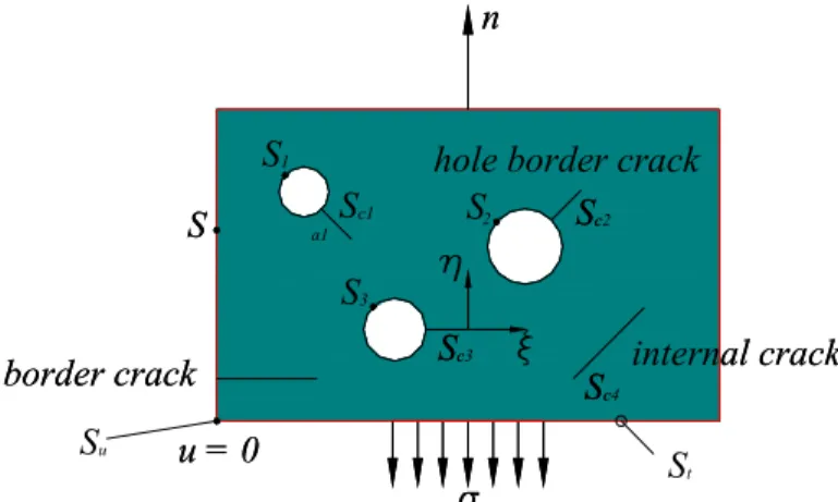
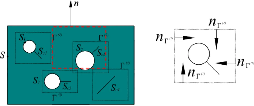
Figure 1 illustrates the problem to be analyzed using the Splitting Method. The two-dimensional linear elastic domain Vc has a boundary S divided into two non-intersecting complementary parts
Su and St(S = StUSu and St∩Su = ø) on which restrictions over displacements and loading can be
prescribed, respectively. The domain contains holes with cracks, an internal crack and a border crack and is submitted in its boundary St to a tensile load.
Figure 1: Two-dimensional domain containing holes and cracks.
Assuming that in Su the displacement vector u is prescribed, the equations governing the
equi-librium condition and the static boundary conditions of the problem are:
∆ on Vc (1)
̅ on St (2)
on Sc1, Sc2, Sc3 and Sc4 (3)
where Δ(.) is the Laplacian operator. In fact, the first condition is a condensed form of representing Lamé’s equations, in which the geometrical characteristics of deformations and the elastic properties of the material are implicit. Equation (2) is a boundary condition making the stress tensor T and the applied loading compatible. In particular, Equation (3) means that the crack surfaces are trac-tion free.
n
internal crack
border crack
hole border crack
S
S
c1S
1a1
S
S
3u = 0
n
internal crack
border crack
hole border crack
S
S
c1S
1a1
S
S
3u = 0
In the Splitting Method, the above problem is split into a fundamental global problem ( ) and into additional global sub-problems ( ) and local sub-problems ( ), whose number is equal to J, described in detail in the following part. The basic aim is to find a stress vector solution t at the crack faces such that:
with 1 k J (4)
where and are stress vector solutions at the crack lines obtained from the global sub-problems and , respectively, and is the stress vector prescribed at the crack faces in the local sub-problem .
2.1 The Global Sub-Problem
The global sub-problem is basically the original given problem domain, without cracks but un-der the prescribed loading and boundary displacements. However, identification lines are placed in coincidence with the lines of the original cracks. From the results of the analysis, traction vec-tors will be computed corresponding to those lines.
The governing equations of this type of sub-problems are:
∆ on V(uncracked domain) (5)
The main features of this sub-problem are: i.Prescribed displacement components:
on Su; (6)
ii.Prescribed external loading:
̅
on St; (7)
iii.Null traction vector along each one of the internal hole boundary Si:
onSi. (8)
Due to the simplicity of this sub-problem, a coarse mesh can be adopted. In fact, it is suitable to adopt a refinement in the mesh only to ensure some accuracy in stresses around the holes and identification lines corresponding to the original cracks. Therefore, local enrichment of the approxi-mation may be exempt, by setting up a situation in which GFEM/XFEM coincides with FEM.
Since the length, position and direction of each crack is known, the traction vector can be com-puted in the identification lines using the solution of this global sub-problem. Moreover, as the nu-merical solution provides components of the traction vector at some arbitrary points along the line
Sci, a continuous approximation of these components can be recovered by means of interpolation.
2.2 The Local Sub-Problem
The basic aim of this sub-problem is to compute the Stress Intensity Factors(SIFs) at each crack tip. As is shown later, in the context of the GFEM/XFEM, by using singular functions as local enrichments of the approximated solution, it becomes feasible to consider the effects of the singular-ities without demanding an excessive mesh refinement.
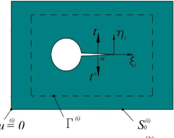
In each local sub-problem, only one crack is considered. This crack may be an internal crack or a hole with a crack, as depicted in Figure 2. Surrounding the crack or the crack and hole, an arbi-trary rectangular contour should be made, hereby represented as Г . It is important to mention that Г cannot intercept other cracks.
In each sub-problem, a set of internal pressure loads is applied to the crack surfaces, using the same normalized polynomial basis (i.e., each component has a maximum unitary value) used in the global problem to identify the continuous traction vectors along the crack lines. Finally, for each component of the polynomial basis, the displacement field and the traction vector t(i) along Г are also computed, as well as the SIFs at the crack tip.
Figure 2: Local Sub-Problem .
The governing equations of this type of sub-problem are:
∆ on (sub-domain containing the holewithcrack set or crack) (9)
i.Prescribed displacement field in , aiming to avoid rigid body movement of :
on ; (10)
ii.Null traction vector at the hole border:
on Si; (11)
iii. Traction vector applied at the faces and of the crack i of length ai: the components of
this vector are polynomial functions of the natural coordinate :
∑ , ⁄ on , (12)
-u = 0
t
+
t
ai
(i)
S
0 (i) (i), ⁄ on (13)
where:
⁄ ⁄ , , , (14)
Polynomial basis with components of order 0, 1 or 2 were adopted. It is clear that any approx-imation function will be represented as a linear combination using elements that belong to this set.
Some comments about the boundary conditions are worthwhile. As observed by Andersson and Babuska (2005), any boundary conditions can be used, provided rigid body movements are avoided. As was mathematically proved by the same authors, although the Stress Intensity Factors and the results on the Г contour are affected in the local problems, the final result will not be changed after the superposition
2.3 Additional Features of Sub-Problems
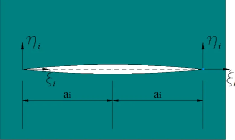
Firstly, it is important to focus on how to apply internal pressure to the internal crack surfaces. Depending on its geometry, each internal crack can be divided into several line segments, which is convenient, particularly if the crack is not straight, therefore presenting a more complex geometry. For instance, in Figure 3, the crack is optionally composed by two equal segments of lengths ai.
Figure 3: Crack i subdivided into two segments.
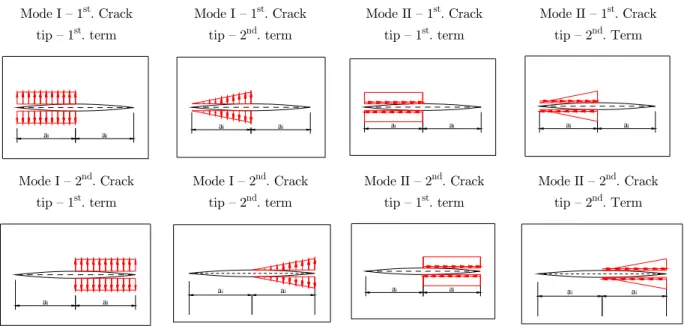
Once the subdivision of the crack line is made, when defining the local problems, each segment is treated as a crack line, and hereafter will be indicated as Sci. As shown in Figure 4, an internal
load must be applied to each Sci. Note that in addition to the conventional mode one, cases of
Mode I – 1st. Crack tip – 1st. term
Mode I – 1st. Crack tip – 2nd. term
Mode II – 1st. Crack tip – 1st. term
Mode II – 1st. Crack tip – 2nd. Term
ai ai a
i ai ai ai ai ai
Mode I – 2nd. Crack tip – 1st. term
Mode I – 2nd. Crack tip – 2nd. term
Mode II – 2nd. Crack tip – 1st. term
Mode II – 2nd. Crack tip – 2nd. Term
ai ai
ai
ai
Figure 4: Applied load on the Sci line.
2.4 On the Г Contour
The Г contour is a rectangular polygon completely enclosing the crack. For each local sub-problem , the displacements and stress fields must be identified at each node of this contour. There must be a sufficient number of nodes in the Г contour in order to ensure the accuracy for the computed displacement and stress fields. However, an excessive number should be avoided in order to reduce the costs in terms of mesh refinement in the correspondent sub-problem .
2.5 The Global Sub-Problem
The Global Sub-Problem is geometrically similar to . Therefore, geometry is described with-out cracks, but the same boundary conditions of the are considered. However, only the dis-placement fields and traction vectors identified in Г of the correspondent local problem are imposed as jumps on . It is important to note that the number of global sub-problems coincides with the number of local sub-problems.
The governing equations of this type of sub-problems are:
∆ on V(un-cracked domain) (15)
In addition, the main features of this type of sub-problem are:
i.Prescribed displacements, which are the same ones as the sub-problem :
on Su (16)
ii.Prescribed null traction vector in St and in the hole borders:
on St, (17)
ai
on Si (18)
Finally, it is very important to highlight the “jumps” that must be prescribed: iii.“Jump” in the traction vector on the Г :
on Г (19)
iv. “Jump” in the displacement field on the Г :
on Г (20)
where and are obtained from the solutions of the local problems . The symbol [•] pre-sented in Equations (19) and (20) denotes jumps in the directions, shown in Figure 5. Accord-ing to condition (20), the displacement field is then imposed in the correspondent sub-problem as a local “jump” in displacements. Analogously, as indicated by Equation (19), the stress field is imposed as a “jump” in forces in the same sub-problem . It is clear that nodes must be posi-tioned in sub-problems to allow the application of both results.
Figure 5: Global Sub-Problem : -directions.
The most important aim of this type of sub-problem is to evaluate the corrections in the solu-tion of the global problem , by taking into account the influence of one crack on another. The solution to the original problem cannot be solved only by the superposition of solutions of the global problem and the local sub-problems. If so, there would be discontinuities along the lines corre-sponding to the Г contours.
2.6 Assemblage of the Problems. Coefficients Provided by and
In the given problem , the traction vector must be null in the crack surfaces. This can be ex-pressed through a weighted residual form, using each component of the approximation basis accord-ing to the followaccord-ing relation:
. ⁄ with j2= 1,…,J (21)
n
S
S
1S
2n
S
S
1S
3S
c1S
c3S
c2S
c4(1) (2)
(3)
(4)
n
(1)n
(1)n
(1)where t is given by Equation (4). In addition, ⁄ is the weight function, taken as one of the components of the polynomial basis functions, as shown in Equation (14).
The traction vector contributions can be represented using ⁄ as follows: i.Global sub-problem :
∑ , . ⁄ , with (22)
ii.Local sub-problem :
∑ . ⁄ , with (23)
iii. Global sub-problem :
∑ ∑ . , . ⁄ , with (24)
where M is the number of local (or global) problems and J is the number of terms of the approxi-mation basis.
It is worth mentioning that a single “α” coefficient for each local problem and the correspondent global problem as a result of the analysis will be computed.
The “ ” coefficients must be organized as a vector composing the unknown vector solution of the linear system. The “b” and “c” coefficients can be previously identified using the results of the global sub-problems and , respectively, by means of the LSM.
Remark: so far, in order to make it easier to understand the text, only Mode I has been
consid-ered.
By substituting equations (22), (23) and (24) in Equation (21), the result is:
, . ⁄ . ⁄ . , . ⁄ . ⁄ (25a)
or:
, . , . ⁄ . ⁄ (25b)
Finally, the following system of equations can be assembled as a function of coefficients “α”:
. (26)
where [GI] is the General Influence matrix.
2.7 Assemblage of the Linear System on the “α” Coefficients Considering Multiple Cracks
In this section, the assemblage of the linear system for many internal cracks is described. The variables and constants used in this section are:
1.Number of cracks: I;
3.Number of segments of each crack: 2;
4.Number of local sub-problems (and global sub-problems): 2 · 2 · I · J = 4IJ
Remark: the number of local sub-problems must be multiplied by 2 in order to consider the two
opening modes. Although two segments for each crack are considered here, the extension for more than two segments is straightforward.
The following expressions are obtained by using Equation (25b):
1.First tip, mode I:
, . , . , , ⁄ . , , ⁄ (27)
2.First tip, mode II:
, . , . , , ⁄ . , , ⁄ (28)
3.Second tip, mode I:
, . , . , , ⁄ . , , ⁄ (29)
4.Second tip, mode II:
, . , . , , ⁄ . , , ⁄ (30)
with j2 = 1…J in all equations.
Concerning internal cracks, some comments are worth mentioning with regards to Equations (27)-(30). As there are at most 2 crack tips, it does not matter which crack tip is chosen as the first or the second one. For each one, there is an associated segment, in which the load is applied (see Figure 4). Equations (27)-(30) show how to consider the influence of each generated sub-problem and its respective load system over both crack tips.
For example, if we consider the first segment of the first crack, Equations (27)-(30) become:
, . , . , , ⁄ . , , ⁄
, . , . , , ⁄ . , , ⁄
, . , . , , ⁄ . , , ⁄
and, for Mode II:
, . , . , , ⁄ . , , ⁄
, . , . , , ⁄ . , , ⁄
, . , . , , ⁄ . , , ⁄
(31b)
The General Influence matrix [GI] can be divided into two sub-matrices:
(32)
where:
1. contains the terms related to the local sub-problems; 2. contains the terms related to the global sub-problems. The matrix, considering all cracks, is presented in the sequel:
,
,
,
, ⋱
,
,
,
(33)
where:
1. is a null matrix of order J x J;
2. , is the matrix of order J x J, related to the first crack tip of crack i in Mode I. The , and , component matrices are described in detail in the sequel:
,
, , , ,
, , , ,
, ,
, ,
, , , ,
⋱
, ,
, , , , , , , , , , , , , , , , , ⋱ , , (34b)
The matrix takes into account the effects of each crack on the other cracks. For example,
,, refers to the effects of the load applied to the first segment of the first crack, normal to
crack surface, related to Mode I (superior index), over the traction in the same segment, related to Mode I. , , refers to the effects of the load applied on the first segment of the first crack, tan-gential to the crack surface, related to Mode II (superior index), over the traction in the same seg-ment. ,, refers to the effects of the load applied on the second segment of the first crack, nor-mal to crack surface, related to Mode I (superior index), over the traction in the first segment of the first crack tip, related to Mode I, and so forth.
,, is described in detail in Equation (35):
,, , ∙ , , , , , ∙ , , , , , ∙ , , , , , ∙ , , , , , ∙ , , , , , ∙ , , , , , ∙ , , , , , ∙ , , , , ⋱ , ∙ , , , , (35)
is presented in the sequel, in Equation (36).
,, , , ,, ,, ,, , , ,, ,, ,, , , ,, ,, ,, , , ,, ,, ,, , , ,, ,, ,, ,, ,, , , ,, ,, ,, ,, ,, ,, ,, ,, ,, ,, ,, ,, ,, ,, ,, ,, ,, , , ,, ,, ,, ,, ,, ,, ⋱ ,, (36)
, ∙ , , , ,
, ∙ , , , ,
, ∙ , , , ,
, ∙ , , , ,
, ∙ , , , ,
, ∙ , , , ,
, ∙ , , , ,
, ∙ , , , ,
, ∙ , , , ,
, ∙ , , , ,
, ∙ , , , ,
(37)
3 COMPUTATIONAL ASPECTS
In order to construct a computational framework to test the combination of the Splitting Method with the GFEM/ XFEM, a complete code had to be created from the mesh generation to the solu-tion of the linear system of equasolu-tions providing the “ ” coefficients of the Splitting Method. A brief review of the GFEM/ XFEM followed by the main idealized and implemented procedures of the computational code is described in this section.
3.1 A Brief Review of GFEM/ XFEM
enrichment strategies of the GFEM/ XFEM to improve the results, therefore avoiding excessive mesh refinement. Hence, close to the crack tips accurate results for the Stress Intensity Factors can be obtained, which are intrinsically derived from the good precision of the stress and displacement fields in its proximity.
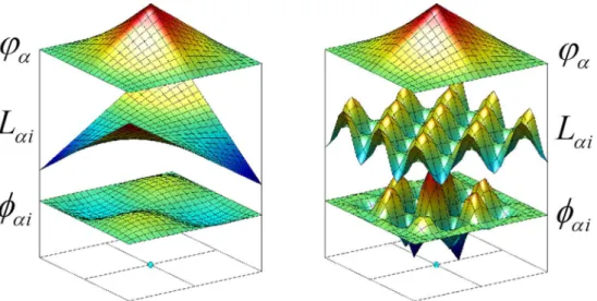
The main difference between the standard FEM and the GFEM/ XFEM is in the definition of the shape functions. In GFEM/ XFEM, the shape functions ϕ i are defined locally in a domain ω called a cloud or patch (the set of elements that have a common vertex node). Inside each cloud, the shape functions are constructed by the product between the so-called enrichment functions L i
and the linear Partition of Unity (PU) functions belonging to the elements in the cloud and at-tached to the vertex (φ ). Therefore:
i
L
i
(38)where identifies the nodal cloud and i = 1,…,nl and nl is the total number of enrichment func-tions adopted for each cloud.
Figure 6 illustrates the construction of a GFEM/ XFEM shape function in a two-dimensional domain.
Figure 6: Representation of a GFEM/ XFEM shape function. Here the FEM shape function, φ is the function at the top and the enrichment function, Li is the function in the middle.
The picture on the left depicts a polynomial enrichment function and the picture on the right shows a non-polynomial enrichment function. The GFEM/ XFEM shape function,
ϕi is the resulting shape function shown at the bottom.
Adapted: Kim, Duarte and Proença, (2009)
1 1 2
ˆ n n nl i i
i
u u b
(39)1 1 2
ˆ
n n nl i ii
v
v
c
(40)where u and v are parameters associated with usual degrees of freedom of finite elements, b and
c are additional nodal parameters introduced by enrichment.
In particular, aiming to improve the results in the crack tip neighborhood, the set of enrichment functions hereby adopted is defined as follows:
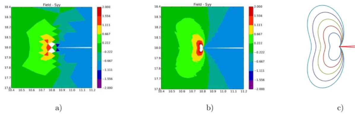
This set of functions can reproduce the Westergaard Complex Stress Functions. The main bene-fit of using GFEM/ XFEM is illustrated in Figure 7.
a) b) c)
Figure 7: Comparison between the yy components in the proximity of a crack tip
obtained from: a) Standard FEM; b) GFEM/ XFEM; c) Analytical solution.
Figure 7 depicts the yy stress component obtained from the analysis of a Local Sub-Problem
defined in the proximity of a crack tip. Both standard FEM and GFEM/ XFEM results are com-pared. The benefit of using the GFEM/ XFEM is clear. Obviously, the same mesh was adopted in both analyses.
More information about the GFEM/ XFEM are available in recent reviews found in Belytschko
et al (2009) and Fries and Belytschko (2010).
3.2 Procedures Associated to
This is the simplest among the problems concerning the Splitting Method. However, two idealized computational procedures are related to it. The first one aims to generate an unstructured mesh composed by triangular elements. For this mesh generation, the available package for Python® named MeshPy® was used. This package can generate an efficient triangular or tetrahedral mesh.
} sin 2 cos , sin 2 sin , 2 sin , 2 cos ,1 {
r r r r
However, only a triangular mesh generation was used in this work. To better explore the MeshPy®, some restrictions must be provided to the program before starting the analysis and mesh genera-tion. The most important is to insert additional nodes: it may be necessary to indicate the regions where additional nodes must be concentrated, especially at the boundary of the plate or at the edg-es of the holedg-es. It is important to mention that it is sometimedg-es necedg-essary to refine the medg-esh close to the crack lines Sci, even in problems, especially when the stress distribution is irregular.
In the developed program, optionally the mesh can be defined manually when global problems are considered. This option is advisable when there are no holes in the problem and the geome-try is relatively simple and, therefore, the adopted mesh is also simple.
It is very important to stress that the MeshPy® generates a mesh with a Constant Stress Tri-angle (CST), therefore with only 3 nodes. However, in the developed program, the created CST to the Linear Stress Triangle (LST) can also be transformed by adding intermediate nodes at the sides of the triangle. In this paper, the LST is optimally indicated for global problems and . Con-sidering the local problems , only CST must be used due to the use of enrichment strategies of the Generalized Finite Element Method.
The second idealized procedure aims to approximate the traction vector taking local values as a reference computed at some points placed along the crack line Sci. In fact, this procedure consists of
a collection of simple functionalities. The most important functionality is responsible for finding out the stress vector components.
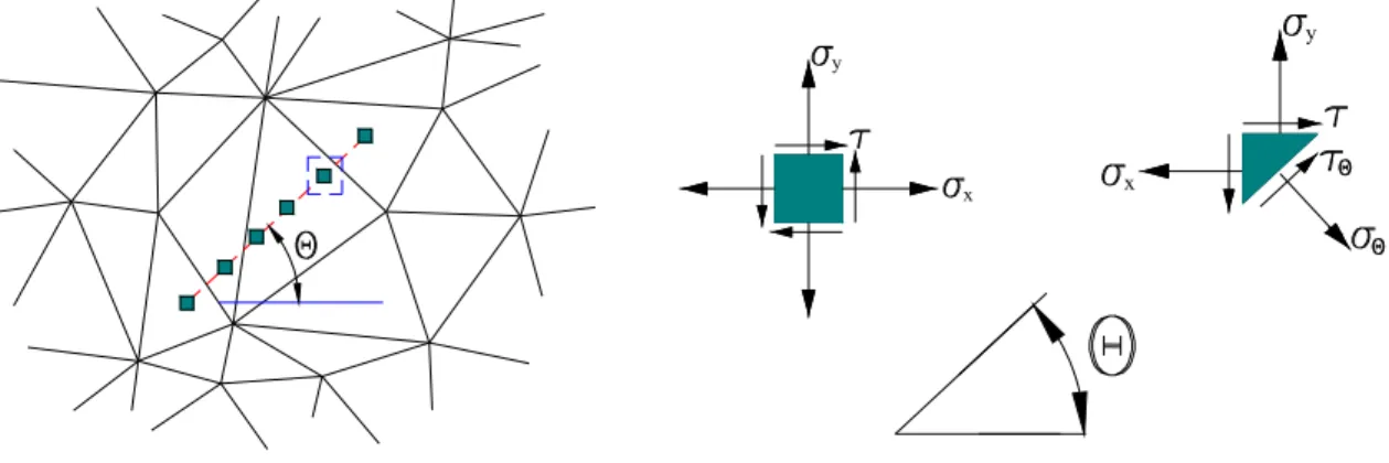
In short, after determining the element to which the point belongs, the next step is to recover the stress tensor components ( x, σy, xy) associated to the reference Cartesian axis. Figure 8 depicts
a small region of the mesh where the crack is inserted, as well as points distributed on the crack line.
Figure 8: Evaluation of the stress tensor at a given point of the mesh.
The squares on the crack line depicted in Figure 8 are points where the stress tensor will be evaluated. The stress components θ and θ, respectively normal and tangential to the crack line at the point, are easily evaluated using the well-known relation:
(41)
y
x
y
It is clear that angle θ refers to the crack angle, as shown in Figure 8.
For each point placed in the crack line Sci, this process is repeated computing the two stress
components. Finally, by using the Least Square Method, an approximation function for θand an-other for θ is determined. Each approximation function is expressed as a linear combination of monomials of order m.
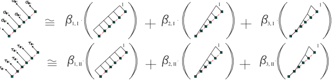
Figure 9: Approximation of the components θand θ along the crack by means of a polynomial function.
In Figure 9, the crack in Figure 8 and its values of components θ and θ in six points are re-produced. As also exemplified in the same figure, the approximation functions are constructed by using a polynomial basis of order 2, for example. The coefficients 1,I, 2,I , 3,I , 1,II , 2,II and 3,II
are obtained using the Least Square Method.
This method is also used in global problems .
3.3 Procedures Associated to the Local Sub-Problems
Fracture mechanics concepts are involved in this sub-problem. Therefore, all the most important procedures hereby idealized are related to modeling the crack and calculating the J Integral. In particular, it is important to note that the J Integral includes the crack surfaces in its paths.
3.3.1 Mesh Generation for Local Problems
The mesh generation in the problems includes the creation of nodes at the external boundary, as well as at the Г contour and along the crack faces. In addition to the creation of the nodes, the procedure includes routines for mesh refinement close to the crack tips and the Г contour.
The shapes of the internal Г contour and external boundary of the problem can be chosen arbi-trarily. However, in order to make the computational development easier, the rectangular geometry was chosen, as shown in Figure 10.
As discussed before, the Г contour must enclose the crack totally and, once existent, the hole with the crack as well. Nevertheless, the respective lengths are arbitrary. In the developed proce-dure, the length of the contour can be defined a priori on the basis of the length of the crack.
It is important to stress that the crack position and its length are the same as proposed in the original problem, but the external boundary and Г contour are defined by the code during the anal-ysis. Particularly over the Г contours, there must be a sufficient number of nodes in order to ensure
1 2
3 4
5 6
1, I
1 1 1
.
2, I. 3, I .
1 2 3
4 5 6
1, II
1 1 1
.
that the results are accurate for the vector stress and displacement fields (these results will be pre-scribed in the problems as jumps in stress and displacements, respectively).
Figure 10: Automatic generation of the nodes at the external boundary and Г contour.
To distribute the nodes at the crack faces, the process may be more complex, considering that the geometry of the crack can be polygonal. Figure 11 illustrates the main steps for the creation of the nodes in a crack with 3 segments, for instance.
Step 1: Initial and final nodes Step 2: Nodes at intersections of the incision lines
Step 3: Intermediatenodes
Figure 11: Steps of the automatic generation of the nodes at crack surfaces.
In the first step, two nodes are inserted at the ends of the crack. In the second step, pairs of nodes are created at the ends of the line segments defined by the bisectors of the corner angles formed by two consecutive crack lines. Finally, in the third step, the additional nodes are distribut-ed along the crack faces describdistribut-ed by joining the nodes defindistribut-ed in the previous steps.
To create the set of nodes at crack faces, each face should be subdivided according to the sub-division rate defined a priori by the user. In the subdivision process hereby adopted, the distribu-tion of nodes along a segment of a crack face follows a geometric rate. More details about this as-pect can be found in Cotta (2016).
Figure 12: Refinement at the crack tip.
The exemplified refinement at the left crack tip is shown in Figure 12. It can be observed that at each level of refinement, 9 nodes were created including the ones already positioned at the crack faces. However, as already mentioned, the number of nodes and levels are arbitrary.
The final result of the node generation is illustrated in Figure 13.
Figure 13: Final result after generating initial nodes.
It should be mentioned that the procedure is also valid to create nodes around the right crack tip.
The remaining nodes needed to generate the mesh are automatically created by the MeshPy®. It is also important to address some comments about the creation of nodes when holes with cracks are considered. Although the cracks do not appear in the global problems, the holes associat-ed to them must be modelassociat-ed in these problems. It is well known that the stress fields experience perturbation at the edges of the holes. To take this perturbation into consideration, the cracks asso-ciated to the holes are modeled using at least two “incision lines” or Sci segments. To exemplify,
consider the crack associated to a hole shown in Figure 14a. The hole is centered at the initial point of the first segment, and its radius is smaller than the length of the referred segment, as shown in Figure 14b. It is important to note that the second segment can be dealt with as a segment pertain-ing a crack without associated holes.
1st level 2nd level
a. Hole with crack to be modeled b. Model of nodes from the cracks associated to the holes generated
Figure 14: Modeled crack and associated hole.
Remark: to make it easier to understand, the opening of the crack has been amplified, as shown
in Figure 14b. In the developed code, the opening is very small and thus, the discrepancy between the crack and the adopted model is not so significant.
Obviously, the length of the first segment is greater than the radius of the associated hole. It is also important to stress that the load in this segment must be applied only at the region that corre-sponds to the crack surface, as indicated in Figure 14b.
It seems clear that the Stress Intensity Factors must be calculated only at the tip of the second segment.
3.3.2 Crack Face Loading
The last procedure refers to loading at the crack surfaces of the local sub-problems. For an explana-tion of this procedure, let us consider Figure 15.
a. Generated Mesh b. Amplified region around the upper
crack surface of the first segment
Figure 15: General aspects of the procedure to apply the loads at the crack surface.
In Figure 15a, the unstructured generated mesh is shown. It is worth noting that the resulting mesh refinement around the left and right crack tips may have different results.
first segment Sci second segment Sci
region of the first segment where the loading must be applied
1st. Crack tip 2nd. Crack tip
The procedure for applying the loads to the crack faces consists of the following steps:
1.Selecting the nodes positioned at the crack faces, in the segment referred to the crack line where the load must be applied. In Figure 15b, only the upper crack surface of the first seg-ment is shown. It is clear that the procedure is analogous on the opposite surface;
2.For each pair of subsequent nodes that are on the same side of the crack face, the element containing these nodes must be identified, as exemplified in Figures 16a and 16b.
a. Load applied in the first segment of the upper crack surface
b. Detail of the applied pressure load in the element highlighted in Figure 16a
Figure 16: Details of the procedure to apply the loads to the crack surface.
3.A distributed load must be applied. In Figure 16b, the element highlighted in Figure 16a is shown. The values of pyi and pyf are defined considering the proportion of the node distances to the crack tips, as follows:
; (42)
where:
1.li: distance between the initial node (i) up to the first crack tip;
2.lf: distance between the final node (f) up to the first crack tip;
3.lT: total length of the first segment;
4.j: degree of polynomial. In the developed program, j can assume the values 0, 1 or 2.
3.4 Procedures Associated to Global Sub-Problem : Imposition of the Boundary Conditions
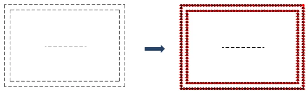
Related to the global sub-problem , there are two important procedures idealized in the compu-tational framework. The first one is the same cited in Section 3.2, aiming to evaluate the stress field in the points positioned along the crack line prescribed in the original problem. The second proce-dure is related to the imposition of the “jumps” in displacements and tractions in the Г contour.
In order to do this, first of all, the option hereby adopted was to set node pairs as close as pos-sible following the whole Г contour. Each pair of nodes must be very close to each other in order to ensure the accuracy of the results as depicted in Figure 17. However, if such a relative distance δ is set excessively small, MeshPy® cannot identify the strip between the two contours and, therefore,
i f
pyf
pyi
does not generate a mesh inside that region. In fact, for each problem to be solved, the distance δ should be set. As a rule of thumb, a reasonable value for δ must be of the order 10-1 of the dis-placements to be prescribed as “jumps”. This rule was set after several numerical experiments aim-ing to reach a reasonable value that was feasible for mesh generation and maintainaim-ing accuracy in the results.
Г contour in the Pair of nodes and Δ distance
Figure 17: Region close to the Г contour in the .
Once the pairs of nodes are defined along the Г contour, the traction vector must be imposed only in one line of nodes of each pair. In the analysis hereby performed, it was chosen to impose this condition in the internal node, but this is arbitrary. To impose the jump in displacements, the pen-alty method can be used.
3.5 J Integral
Aiming to evaluate the Stress Intensity Factors (SIFs), Rice (1968) formulated the J Integral con-cept. It addresses a path-independent line integral whose value corresponds to the decrease in po-tential energy when an increment of crack extension occurs. The J Integral applies either linear or nonlinear elastic materials. The J Integral can be represented by:
∙
Г (43)
or, in an alternative expression, conveniently using indicial notation, as:
n ∙ u
Г (44)
where:
1.W is the strain energy density:
, (45)
pair of nodes
δ
2.The traction vector T is a force per unit area acting at a point with respect to a plane defined by a normal versor n, as shown in Figure 18.
(46)
Figure 18: Arbitrary path Г enclosing a crack tip. Traction vector T and normal vector n to the segment ds.
It is important to note, as shown in Figure 18, that the path of integration Г is not necessarily circular. However, in this work a circular path was adopted in order to take advantage of some characteristics of the polar co-ordinates. Therefore:
cos (47)
The J Integral can be viewed as a measure of an amount of energy comparable to the energy
re-lease rate G, or else, G=J. It is also important to remember the relations between J Integral and the Stress Intensity Factors:
(Plane Stress) (48a)
(Plane Strain) (48b)
To evaluate the J Integral numerically, a particular procedure is hereby proposed. First of all, consider a circular path of integration around the crack tip. This path is divided into 4 segments. Next, each segment is further subdivided into 3 segments. Therefore, there are 4 segments, each one with 2 intermediate points. The reason is due to the option of mapping an arc of circumference through a polynomial of order 3. In Figure 19a, the following segments can be observed: i) 0-1-2-3; ii) 3-4-5-6; iii) 6-7-8-9; iv) 9-10-11-12.
Remark: The finite element mesh adopted to discretize the neighborhood of the crack tip is
omitted in the figure to focus only on the integration path. The axes depicted in the figure are local axes.
Next, each segment is mapped onto a dimensionless straight line segment, as shown in Figure 19b. It is important to follow the integration direction, as depicted in Figure 18. Thus, for the first segment (0-1-2-3), the point labeled “0” is attached to co-ordinate ξ = -1.0, the point labeled “1” is
x y
o
ds
attached to co-ordinate ξ = -1/3, the point labeled “2” is attached to co-ordinate ξ = +1/3, and the point labeled “3” is attached to co-ordinate ξ = +1.0, and so on for the other segments.
a. Circular path subdivided into segments b. Natural coordinates
Figure 19: Path of integration.
In the sequel, the integration along path Г is substituted by a sum of integrals along each seg-ment, as shown in Equation (49):
∙ n ∙ u
Г ∙ n ∙
u
Г (49)
where nseg is the number of segments in which path Г is divided. In the example shown in Figure 19, nseg is equal to 4. Afterwards, each integral on the right hand side of Equation (49) is made using the natural co-ordinate system defined above and shown in Figure 19b:
∙ n ∙ u
Г ∙ n ∙
u .
. . , . .4 (50)
where Jac is the Jacobian operator relating the natural co-ordinates to the local co-ordinates. Finally, the right hand side of Equation (50) can be substituted by a numerical integration:
∙ n ∙ u
.
. . ∙
u u
. (51)
where:
1.ngp is the number of sampling points of the Gauss quadrature; 2.xi is the ith sampling point;
3.W(xi) is the weight function evaluated in xi.
However, instead of computing Equation (51) directly, it is necessary to divide J in order to ob-tain KI and KII separately. This procedure was presented by Ishikawa et al (1980) and used by
Kzam (2009). According to Equation (52), the J Integral can be separated into two parts:
J
=
J
I+
J
II (52)where:
1.JI refers to Mode I of opening;
2.JII refers to Mode II of opening.
To calculate JI, the displacements and stress fields are replaced by auxiliary fields uI and I,
re-spectively, according to Equations (53) and (54):
(53)
(54)
In Equation (53), , is the displacement field at a symmetric point of the point that was analyzed in relation to the local x-axis. Similarly, in Equation (54), , is the stress field at the samepoint. For example, in Figure 19a, point “12” is the symmetric of point “0”, point “11” is the symmetric of point “1” and so on. Obviously, the reciprocal is also true.
Furthermore, to evaluate JII, the auxiliary fields are given by:
(55)
(56)
In Figures 20 and 21, the results of the operations correspondent to Equations (53)-(56) are pre-sented for an arbitrary point P and its symmetrical point P’.
Mode I
Figure 20: Symmetric and anti-symmetric components of the displacement field for Mode I.
x y
o
11,P I 22,P
I
12,P I
22,P' I
12,P' I 11,P'
I P
P' x
y
o
u1, P I
u2, P I
P
P' u1, P'I
Mode II
Figure 21: Symmetric and anti-symmetric components of the displacement field for Mode II.
Analyzing Equations (53)-(56), and by observing Figures 20 and 21, it can be concluded that for Mode I:
1. , , ´
2. , , ´
3. , , ´
4. , , ´
5. , , ´
And, for Mode II:
6. u, u , ´
7. u , u , ´
8. σ , σ , ´
9. σ , σ , ´
10.σ , σ , ´
An important aspect that must be mentioned is that loads are applied to the crack surfaces and their contribution must be considered in the calculus of the J Integral. To address this issue, the solution proposed by Karlsson and Bäcklund (1978) was hereby adopted. Accordingly, a decomposi-tion of the J Integral is assumed as:
J = J
cp+ J
scs+ J
ics (57)where Jcp is the contribution of the circular path to the J Integral and Jscs, Jics are the contributions
of the upper and lower crack surfaces, respectively.
The procedure to compute the values of Jscs and Jics is identical to that described above for the
calculus of the J Integral in the circular path, and each crack surface is analogously divided into 3 segments and then mapped into a linear segment.
The procedure to evaluate the contribution of the crack surfaces for the JIntegral was treated separately in this paper in order to emphasize some important features:
1.Most of the programs containing routines for calculating J require a specification of an inte-gration path around the crack tip from the user, assuming that the crack surface is traction free; x y o 11,P II 22,P II 12,P II P 22,P' II 12,P' II 11,P' II P' x y o
u1, P II
u2, P II
P
P' u2, P'
II
2.The error in the calculus of the JIntegral considering the crack surfaces can be strongly af-fected by the accuracy of the stress field very close to the crack tip. Therefore, special care must be taken aiming to improve the accuracy in that region, for example, by refining the mesh or, as hereby adopted, by using enrichment strategies.
It is worthwhile to mention that the code using the J Integral was implemented in order to evaluate the referred value in local problems PLKs. After solving these problems, the developed program assembles the path, calculates the J Integral and stores its value as another output of the respective local problem. Thus, the analysis can be done without interruptions in order to evaluate the J Integral using another program. Further, a future improvement of the program to consider propagation issues demands an automatic calculus of a parameter that indicates the direction and rate of propagation.
4 NUMERICAL EXAMPLES
Two examples are presented to illustrate the Splitting Method. The first example is a domain em-bedded one with a slanted crack and a hole with a crack. In the second example, there are two cracks: the first one has an arbitrary shape and the second one has a horizontal straight crack.
For both examples, the Poisson’s ratio is 0.3 and the Young modulus is 1000.
4.1 Example 1: Domain Containing a Slanted Crack and a Hole with a Crack
This example aims to demonstrate the ability of the developed framework to account for mixed opening mode and cracks associated to holes.
The geometry of the problem is depicted in Figure 22a. The tips of the cracks are labeled with the capital letters A, B and C. The reference values were obtained by using the Franc2D® program,
and the mesh adopted to assess the reference solution is shown in Figure 22b.
a. Geometry b. Mesh used in Franc2D®
Figure 22: Domain with embedded slanted crack and hole with crack.
20.0
20.0
(16.0,10.9)
(14.0,9.1)
y
x O
(7.0,10.0) 4.0
10
.0
1.0
Regarding the local problems, the meshes adopted can be seen in Figures 23a and 23b. Some stress fields of interest obtained in the analysis of the local problems are also shown in Figures 23c and 23d.
a. Used mesh to analyze the crack attached to a hole b. Used mesh to analyze the slanted crack
c. Stress component yy d. Stress component yy
Figure 23: Adopted meshes and stress fields of interest.
A polynomial basis up to the quadratic approximation was used to analyze the local problems ’s (as well as to recover the stress vector at the crack lines of the global problems ’s). Thus, the number of problems (nop) is:
nop = 4 x 2 x 3 = 24
In relation to the boundary conditions of the local problems, the displacements components (dx
and dy) were prescribed equal to zero at the whole external boundary.
Particularly for the sixtieth local problem (i.e., k = 6), in which the second segment Sci of
the crack is subjected to a constant normal stress component, the stress component yy is shown in
Figure 23c. The same component stress for the second crack and local problem k = 12, in which its first segment is subjected to a constant normal stress component, is shown in Figure 23d.
The SIFs obtained using Franc2D® (for both J Integral and Displacement Correlation
Tech-nique, DCT) and with SCIEnCE code are presented in Table 1.
Crack tip A Crack tip B Crack tip C
KI KII KI KII KI KII
SCIEnCE 2.820 0.0280 1.264 0.968 1.248 0.973
Franc2D® (DCT) 2.815 -0.0219 1.248 1.013 1.201 1.018
Franc2D®
(J Integral) 2.815 -0.0241 1.255 0.967 1.208 0.978 Table 1: SIFs obtained using Franc2D® x SCIEnCE (Splitting Method).
It can be observed that the results obtained using SCIEnCE are very close to those obtained from Franc2D®. It should be noted that even using Franc2D®, there are some discrepancies when
using the J Integral and Displacement Correlation Technique, especially in KII values. Obviously,
since both results were computed numerically, it is reasonable to expect some differences among them.
4.2 Example 2: Domain Containing Cracks with Arbitrary Shapes
In this example, a domain with two cracks is analyzed as shown in Figures 24a and 24b. In order to guarantee the existence of some influence of one crack on the other, a relative distance (3.175 in Figure 24b) was chosen. One of the cracks (crack 1) consists of three segments. In each segment, constant and linear approximations were applied at the crack faces according to Figure 4. There-fore, a total of 24 local and 24 global sub-problems were used.
4 “incision lines”, 2 for each crack. 2 Modes (I and II)
a. Geometry b. Position and dimensions of the cracks
Figure 24: Domain with cracks of arbitrary shapes.
The reference values were obtained from the ANSYS® program. The mesh consisted of 36918
CSTs (Constant Strain Triangles), automatically generated by the program. Quarter point elements were explored close to the crack tip, to provide better accuracy for the Stress Intensity Factors. The component yy of the stress field is depicted in Figure 25a and 25b. This picture refers to the final
results of the original problem.
The results related to the local problems computed using SCIEnCE are presented in Figure 26. The cracks were modeled using 6 incision lines, or 6 Sci segments.
a. Stress component yy b. Amplified region around the crack tip
Figure 25: Stress field of interest around the crack tip.
a. Used mesh in local problems b. Stress component yy
Figure 26: Mesh for local problems and stress field of interest.
The values of KI for crack 1 are shown in Table 2. It can be observed that the results are
rela-tively close to those obtained in the reference problem. Nevertheless, it is worthwhile mentioning that the Stress Intensity Factors are quite sensitive to the ANSYS® program.
Left crack tip Right crack tip ANSYS® SCIEnCE ANSYS® SCIEnCE
712.59 761.45 695.95 698.94
Table 2: KI of crack 1: ANSYS® x SCIEnCE (Splitting Method with GFEM).
5 CONCLUSIONS
In this paper, the Splitting Method was recognized as an efficient method to analyze multi-site damage problems. In these problems, despite the fact that each individual crack is harmless, the combined effects of multiple cracks growing can be disastrous. In order to address more complex scenarios, some improvements for the Splitting Method were proposed, for instance the ones aiming to expand its application to arbitrary polygonal shapes of the crack. On the other hand, enrichment strategies of the approximation avoiding costly mesh refinements were hereby successfully provided by the Generalized Finite Element Method. A computational framework combining the Splitting Method with the GFEM was created involving automatic generation of each sub-problem until the linear equation system was assembled.
The main findings and/or contributions of this work are summarized below.
GFEM efficacy: the good effects of the enrichment used to improve the numerical results could be observed. In particular, the enrichment was more accurate for the local sub-problems, es-pecially when calculating the Stress Intensity Factors.
Implementation of a code to evaluate J Integral: it is possible to state that the
develop-ment of a code that generates an integration path and calculates the J Integral is another contribu-tion of this work. In spite of be very simple, the proposed method consists of a powerful and alter-native tool to provides the SIFs, without directly using the elements of the mesh.
Analysis of domains with cracks of arbitrary shapes and under mixed opening
modes: another important contribution of this work consisted of extending the Splitting Method to
analyse problems containing cracks with arbitrary shapes. Obviously, when cracks with arbitrary shapes are considered, mixed crack opening modes must be also considered. When such modeling is available, complex real-life problems can be analyzed.
As suggestions for future work using the Splitting Method, the following can be highlighted: finding the worst scenario among many possible scenarios of multiple cracks, for instance taking the maximum value of Stress Intensity Factors (SIFs) as the main criterion. In fact, if many cracks are similar, the analysis can be considerably simplified, using only a few local problems to evaluate a large number of possible scenarios.
Finally, the generated code is indeed a very important tool that should be developed in the fu-ture to improve computational efficiency.
Acknowledgements
The authors would like to gratefully acknowledge the Coordination for the Improvement of Higher Education Per-sonnel (CAPES) for the financial support.
References
Alves MM (2010). Splitting Method for Multiple Cracks Analysis. PhD Thesis. The São Carlos School of Engineer-ing, University of São Paulo, (in portughese).
Andersson B, Babuška I (2005) The Splitting Method as a tool for multiple damage analysis. SIAM J. SCI Comput. 26-4.
Babuska I, Andersson B (1996).“A Splitting Method for Fracture Mechanics Analysis.” FFA-TN-1996-27, The Aero-nautical Research Institute of Sweden, Stockholm.
Babuška I, Melenk JM (1995) The partition of unit finite element method. Technical Report BN-1185, Inst. for Phys. Sc. and Tech., University of Maryland.
Babuška I, Melenk JM (1997) The partition of unit method. Int J Numer Methods Eng 40: 727-758.
Barros FB, Proença SPB, de Barcellos CS (2004) Generalized finite element method in structural nonlinear analysis – a p-adaptive strategy. Computational Mechanics, Vol.33, 2, pp 95-107.
Belytschko T, Gracie R, Ventura G (2009) A review of extended/generalized finite element methods for material modeling. Model Simul Mater Sci Eng 17: 24pp.
Cotta IFS (2016). Splitting Method in Multisite Damage Solids: Mixed Mode Fracturing and Fatigue Problems. Doctorate Thesis. School of Engineering of São Carlos. University of São Paulo. www.eesc.usp.br (to appear)
Duarte CA, Babuška I, Oden JT (2000) Generalized finite element methods for three-dimensional structural mechan-ics problems. Comput Struct 77:215-232.
Fries T-P, Belytschko T (2010) The extended/generalized finite element method: An overview of the method and its applications. Int J for Num Methods in Engineering, Vol.84, 3, pp. 253-304.
Ishikawa H, Kitagawa H, Okamura H. (1980) J-integral of mixed mode crack and application. Proc. 3rd Int. Conf. on Mechanical Behaviour of Material. Pergamon Press. Oxford, Vol. 3, pp. 447-455.
Karlsson A, Bäcklund, J (1978). J-Integral at Loaded Crack Surfaces. Int. Journal of Fracture. Vol.14.
Kzam AKL (2009). Formulação dual em Mecânica da Fratura utilizando Elementos de Contorno curvos de ordem qualquer. Master dissertation. School of Engineering of São Carlos. University of São Paulo.
Kim D, Duarte CA, Proença SPB (2009) Generalized Finite Element Method with global-local enrichments for non-linear fracture analysis. Mechanics of Solids in Brazil. ISBN 978-855-85769-43-7.
Kim D, Duarte CA, Proença SPB (2012) A generalized finite element method with global-local enrichment functions for confined plasticity problems. Computational Mechanics, Volume 50, Issue 5, pp 563-578.
Le Tallec P, Domain decomposition methods in computational mechanics. Computational Mechanics /advances, 1, ed J.T. Oden, 1994, p 121-220.
Piedade Neto D, Ferreira MDC, Proença SPB (2013) An object-oriented class design for the generalized finite ele-ment method programming. Latin American Journal of Solids and Structures 10:1267-1291.
Sukumar N, Moës B, Moran B and Belytschko T. (2000) “Extended finite element method for three-dimensional crack modeling”, International Journal for Numerical Methods in Engineering, Vol. 48, pp. 1549-1570.
Strouboulis T, Copps K, Babuška I (2001) The generalized finite element method. Comput Methods Appl Mech Eng 190:4081-4193