Analysis of local AWS and NCEP/NCAR reanalysis data at Lake El'gygtytgyn, and its implications for maintaining multi-year lake-ice covers

(1)

CPD

8, 1443–1483, 2012

Local AWS and NCEP/NCAR reanalysis data at Lake El’gygtytgyn

M. Nolan

Title Page

Abstract Introduction

Conclusions References

Tables Figures

◭ ◮

Back Close

Full Screen / Esc

Printer-friendly Version Interactive Discussion

Discussion

P

a

per

|

Dis

cussion

P

a

per

|

Discussion

P

a

per

|

Discussio

n

P

a

per

Clim. Past Discuss., 8, 1443–1483, 2012 www.clim-past-discuss.net/8/1443/2012/ doi:10.5194/cpd-8-1443-2012

Climate of the Past Discussions

This discussion paper is/has been under review for the journal Climate of the Past (CP). Please refer to the corresponding final paper in CP if available.

Analysis of local AWS and NCEP/NCAR

reanalysis data at Lake El’gygtytgyn, and

its implications for maintaining multi-year

lake-ice covers

M. Nolan

University of Alaska Fairbanks Institute of Northern Engineering, 306 Tanana Loop, Suite 525, Fairbanks, AK 99775, USA

Received: 1 March 2012 – Accepted: 15 March 2012 – Published: 23 April 2012

Correspondence to: M. Nolan ([email protected])

(2)

CPD

8, 1443–1483, 2012

M. Nolan

Title Page

Tables Figures

◭ ◮

Back Close

Full Screen / Esc

Discussion

P

a

per

|

Dis

cussion

P

a

per

|

Discussion

P

a

per

|

Discussio

n

P

a

per

Abstract

We compared 7 years of local automated weather station (AWS) data to NCEP/NCAR reanalysis data to characterize the modern environment of Lake El’gygytgyn, in Chukotka Russia. We then used this comparison to estimate the air temperatures required to initiate and maintain multi-year lake-ice covers to aid in paleoclimate

re-5

constructions of the 3.6 M years sediment record recovered from there. We present and describe data from our AWS from 2002–2008, which recorded air temperatures, relative humidity, precipitation, barometric pressure, and wind speed/direction, as well as subsurface soil moisture and temperature. Measured mean annual air temperature (MAAT) over this period was ₋10.4◦C with a slight warming trend during the

mea-10

surement period. NCEP/NCAR reanalysis air temperatures compared well to this, with annual means within 0.1 to 2.0◦C of the AWS, with an overall mean 1.1◦C higher than the AWS, and daily temperature trends having a correlation of over 96 % and cap-turing the full range of variation. After correcting for elevation di_fferences, barometric pressure discrepancies occasionally reached as high as 20 mbar higher than the AWS

15

particularly in winter, but the correlation in trends was high at 92 %, indicating that synoptic-scale weather patterns driving local weather likely are being captured by the reanalysis data. AWS cumulative summer rainfall measurements ranged between 70– 200 mm during the record. NCEP/NCAR reanalysis precipitation failed to predict daily events measured by the AWS, but largely captured the annual trends, though higher by

20

a factor of 2–4. NCEP air temperatures showed a strong trend in MAAT over the 1961– 2009 record, rising from a pre-1995 mean of₋12.0◦C to a post-1994 mean of₋9.8◦C. We found that nearly all of this change could be explained by changes in winter tem-peratures, with mean winter degree days (DD) rising from₋5043 to₋4340 after 1994 and a much smaller change in summer DD from+666 to+700. Thus, the NCEP record

25

(3)

CPD

8, 1443–1483, 2012

M. Nolan

Title Page

Tables Figures

◭ ◮

Back Close

Full Screen / Esc

Discussion

P

a

per

|

Dis

cussion

P

a

per

|

Discussion

P

a

per

|

Discussio

n

P

a

per

was unlikely to have initiated a multi-year ice cover since 1961 based on simple DD models of ice dynamics. Using these models we found that the NCEP/NCAR reanal-ysis mean MAAT over 1961–2009 would have to be at least 4◦C colder to initiate a multi-year ice cover, but more importantly that multi-year ice covers are largely con-trolled by summer melt rates at this location. Specifically we found that summer DD

5

would have to drop by more than half the modern mean, from+640 to+280. Given that the reanalysis temperatures appears about 1◦C higher than reality, a MAAT cooling of 3◦_{C may be su}_ffi_{cient in the real world, but as described in the text we consider a}

cool-ing of₋4◦C_±0.5◦C a reasonable requirement for multi-year ice covers. Also perhaps relevant to paleo-climate proxy interpretation, at temperatures cold enough to maintain

10

a multi-year ice cover, the summer temperatures could still be sufficient for a two-month long thawing period, including a month at about+5◦C Thus it is likely that many sum-mer biological processes and some lake-water warming and mixing may still have been occurring beneath perennial ice-covers; core proxies have already indicated that such perennial ice-covers may have persisted for tens of thousands of years at various times

15

within the 3.6 M years record.

1 Introduction

This paper explores the relationship between locally measured automatic weather station data and the NCEP/NCAR global reanalysis dataset (Kalnay et al., 1996) for the purpose of understanding inter-annual variations in seasonal trends and how

20

these may relate to lake ice dynamics in a 3 million year long sediment core at Lake El’gygytgyn, Chukotka, Russia. The lake lies inside a 3.6 million year old meteorite impact crater, which has presumably been filling with sediments since the time of the impact. The impact, the crater, the sediment core, and the physical environment are all well-described in a series of prior papers (Belya and Chershnev, 1993; Glushkova,

25

(4)

CPD

8, 1443–1483, 2012

M. Nolan

Title Page

Tables Figures

◭ ◮

Back Close

Full Screen / Esc

Discussion

P

a

per

|

Dis

cussion

P

a

per

|

Discussion

P

a

per

|

Discussio

n

P

a

per

Minyuk et al., 2007; Nolan and Brigham-Grette, 2007; Brigham-Grette, 2009; Swann et al., 2010) and those found in this special issue (Brigham-Grette et al., 2012; De-Conto and Koenig, 2012; Melles et al., 2012; Minyuk et al., 2012). The core contains many proxies for paleoclimate over this time, and many of these proxies suggest that multi-year ice cover may have persisted for thousands of years at a time. One of our

5

goals in this paper is therefore to place some quantitative constraints on the condi-tions necessary to form and maintain such an ice cover, following up on prior related research (Nolan et al., 2003). Here we focus on describing a 7 years data set (2002– 2008) from a local automated weather station (AWS) that we established, determining how well these data compare to the NCEP/NCAR reanalysis (also referred to herein

10

as “NNR” or just “reanalysis”) data, exploring useful trends in these data, and relating these trends to the timing and duration of lake ice cover. A companion paper in this special issue (Nolan et al., 2012) builds on this information by using the self-organized mapping (SOM) technique to explore how synoptic-scale weather patterns drive local weather and how these patterns have changed over time.

15

2 Local automated weather station- description and data quality

We installed a weather station near the outlet of the lake in July 2001 (67.446517◦N 172.186200◦E), as shown in Fig. 1. The station utilized a Campbell Scientific Inc (CSI) CR10x datalogger, powered by a 100 Ah deep cycle battery recharged by a small solar panel. Most measurements were logged hourly, with air temperatures and wind

20

speeds being sampled every minute. There was no telemetry and all data were stored in the logger and backup memory card. The instruments were mostly all standard, sold through CSI:

– two Vaisala HMP45c measured air temperature and relative humidity, at 1.0 m and 3.03 m above ground surface,

(5)

CPD

8, 1443–1483, 2012

M. Nolan

Title Page

Tables Figures

◭ ◮

Back Close

Full Screen / Esc

Discussion

P

a

per

|

Dis

cussion

P

a

per

|

Discussion

P

a

per

|

Discussio

n

P

a

per

– a CSI SR50 sonic ranger was used to measure snow depth, recording values subtracting its own height so that the me,asurement read height above ground,

– a Young AQ Wind Monitor at 4 m

– a barometer (Vaisala),

– a net radiometer (Radiation and Energy Systems Q7.1) at 3.5 m,

5

– six thermistors on a (homemade) calibrated string installed in a pit to depth of 60 cm,

– eight CSI SM615 soil moisture probes installed in a pit to depth of 60 cm,

– a tipping bucket (Texas Instruments) mounted on the ground surface (0.01′′tips). The station had little maintenance from the time it was installed in 2001 to when it was

10

dismantled in March 2009. The day after leaving the site in 2001, the station was shot with a rifle by a local drunk, destroying the logger and the battery. In July 2002, the logger and battery were replaced. In July 2003, the station was downloaded and one loose wire in the 3m air temperature sensor tightened and level checked on appropriate instruments. Battery power began to fail in late winter 2008 causing some gaps but

15

functioned fine once sun returned to this Arctic site, until it again failed in early 2009. It was still recording data when dismantled, though the battery failure that spring had caused the date and time reset to an arbitrary setting. Other than these gaps, the remaining years had at most a few missing time-steps caused by static, low power, or some undetermined cause. Calendar years 2002–2007 therefore had better than

20

99.99 % recovery and 92.8 % in 2008, in terms of hourly time-steps logged.

Individual sensors did not necessarily fare as well as the logging system itself over the recording period. Since we have made these data freely available to the scientific community, what follows is a brief description of quality control of individual sensors and a few sample plots for easy reference. The data from 2002–2003 were described

(6)

CPD

8, 1443–1483, 2012

M. Nolan

Title Page

Tables Figures

◭ ◮

Back Close

Full Screen / Esc

Discussion

P

a

per

|

Dis

cussion

P

a

per

|

Discussion

P

a

per

|

Discussio

n

P

a

per

already in detail in (Nolan and Brigham-Grette, 2007), and the reader is referred there as this paper tries not to repeat much of those analyses but rather add to them. Dis-cussion of the data itself is largely reserved until the next section.

2.1 Air temperature and relative humidity

The 1m AT/RH sensor performed without any issues for the duration of the installation.

5

The 3 m AT/RH failed from 2002 Day 206 at 08:00 LT apparently caused by the socket handle coming loose. This was retightened on 2003 Day 159 18:00 LT. All remaining values seemed within tolerance of ₋40 to +40◦_{C other than gaps caused by logger}

failures in early 2008. None of the probes were replaced or recalibrated during the study period. Comparison plots of the two AT sensors in winters (that is, when there

10

was no solar radiation loading) shows they are within 0.1◦C of each other with a cross-correlation value of over 99 %, which likely means that drift was minimal or both drifted the same amount (likely the former). Summer values (that is, when solar loading was appreciable) did show differences of up to several degrees, but much of this difference is likely real and the remainder due to the differences in solar loading of the

radia-15

tion shields and differences in wind cooling rates. Figure 2 shows the daily minimum, maximum, and mean of the 1m air temperature for the AWS (thin lines). The lowest recorded temperatures are₋40◦_{C due to a limitation of the sensor itself, but inspection}

of the hourly data trends reveals that such temperatures were uncommon and thus clipping was minimal and likely did not affect daily or annual means noticeably. Both

20

RH sensors drifted slightly with time with their maximum recordable range decreasing (Fig. 3), as is typically for these sensors. The range of values is within reasonable expectations, with the largest variability in summer when higher air temperatures sub-stantially a_ffect the absolute amount of moisture the air can carry. Note that in winter, the recorded RH is never fully saturated, and the mean summer RH is approximately

25

(7)

CPD

8, 1443–1483, 2012

M. Nolan

Title Page

Tables Figures

◭ ◮

Back Close

Full Screen / Esc

Discussion

P

a

per

|

Dis

cussion

P

a

per

|

Discussion

P

a

per

|

Discussio

n

P

a

per

2.2 Tipping bucket

The tipping bucket seemed to remain functional until June 2008. Values from 2008 are suspect, as they are anomalously low, with no tips shown throughout July and August even though the soil moisture probes were clearly recording rainfall during this time. The unit was not re-leveled during the study period, so some bias or drift may have

oc-5

curred, but it was still firmly anchored upon removal and no noticeable tilt was recorded at that time. Figure 4 shows annual cumulative rainfall for 2002–2007, revealing nearly a factor of 3 inter-annual difference (73 mm to 200 mm), though the range is consistent with measurements elsewhere in the Arctic (Kane and Yang, 2004). The tipping bucket had no wind shielding, thus these values are probably low by 10–50 %, possibly higher

10

(Yang et al., 2005).

2.3 Wind speed and direction

This instrument seemed to be performing fine until 2005 Day 259 when it apparently blew apart during a 30 m s−1_{wind storm; the unit had previously survived a few dozen}

storms of this magnitude. While functional, there were occasional data gaps likely due

15

to the unit getting stuck by rime, as the gaps only occur during the middle of winter. While functional, no substantial differences in wind speed or direction were noticed compared to the detailed analysis in (Nolan and Brigham-Grette, 2007) of 2002–2003, which indicated nearly all winds coming from the north or south and likely responsible for the orientation and square shape of the lake.

20

2.4 Net radiation

This sensor remained functional throughout the installation duration. However, it is well known that the sensor domes degrade with time, and these measurements should therefore not be used quantitatively after the first year. Also, the unit was never re-leveled after 2003. Towards the end the domes were clearly deteriorated and were

(8)

CPD

8, 1443–1483, 2012

M. Nolan

Title Page

Tables Figures

◭ ◮

Back Close

Full Screen / Esc

Discussion

P

a

per

|

Dis

cussion

P

a

per

|

Discussion

P

a

per

|

Discussio

n

P

a

per

mostly likely cracked, and certainly the desiccant was not functional at all after a year or two. The values stayed pretty consistent year-to-year nonetheless and qualitatively it may be a useful dataset.

2.5 Sonic ranger

The sonic ranger began performing erratically after 2002, but still provided useful

5

(though noisy) information through 2005. After this it appears to be not useful at all. Likely the shielding deteriorated over time and was interfering with the sensor. The cable or its contacts may also have degraded. In any case, take great care in using these data; actual snow depth likely never exceeded 0.5 m, despite recorded values being much higher at times.

10

2.6 Soil moisture

The soil moisture sensors remained functional throughout the installation period and were for the most part within range except for some obvious data drop-outs. We con-verted voltages to volumetric soil moisture using equations from Campbell Scientific for low conductivity soils. The values may not be as accurate as a custom calibration, but

15

the trends are real and water measurements here show very low electrical conductiv-ity (Cremer and Wagner, 2003). It appears in general there is a water table between 20 cm and 40 cm, but in 2006 this table rose to near the surface, froze in place, and then thawed the following summer, as is described more fully in Federov et al. (2012) in this special issue.

20

2.7 Soil temperature

(9)

CPD

8, 1443–1483, 2012

M. Nolan

Title Page

Tables Figures

◭ ◮

Back Close

Full Screen / Esc

Discussion

P

a

per

|

Dis

cussion

P

a

per

|

Discussion

P

a

per

|

Discussio

n

P

a

per

connection at the logger was not solid or the waterproofing at the sensor was damaged. These data are described more fully in Federov et al. (2012) in this special issue.

2.8 Barometric pressure

The barometer seemed to work fine throughout the installation period. As it takes some current to make a measurement, during low battery voltages the values may be lower

5

than actual, especially just after a complete logger brown out, so take some care in winter when interpreting low pressure values.

3 Comparison of local AWS to NCEP/NCAR Reanalysis

One of our main goals in comparing the AWS to the NCEP/NCAR reanalysis data is to then use the reanalysis data to explore trends in variables beyond our instrumental

10

record to better understand the variability in the modern environment. To accomplish this, we extracted the NNR 2-meter temperature for the grid point closest to our site. Of primary interest to core proxy interpretations are air temperatures and precipitation. NCEP/NCAR reanalysis and AWS air temperatures compared well enough that we believe that the reanalysis data is suitable for both numerical lake-ice modeling and for

15

our purposes in exploring synoptic climatology trends in our companion paper (Nolan et al., 2012). Annual means of air temperature and its trend compare well between datasets (Fig. 5, MAAT) especially considering the coarseness of the reanalysis grid, with the AWS recording 0.1 to 2.0◦C colder than NNR, with a mean difference of 1.1◦C from 2002–2007. Figure 2 shows the comparison between daily means of minimum,

20

maximum, and mean air temperatures. The best fit in both means and range is in peak summer, which is ideal for our model of lake ice melt, as ice melt, as we describe later, is more important than ice growth at this location in terms of maintaining perennial ice cover. The extreme lows match best in late-winter through summer, with NNR lows tending to be 5–10◦C colder in fall. The extreme highs tend to fit best in spring-fall,

(10)

CPD

8, 1443–1483, 2012

M. Nolan

Title Page

Tables Figures

◭ ◮

Back Close

Full Screen / Esc

Discussion

P

a

per

|

Dis

cussion

P

a

per

|

Discussion

P

a

per

|

Discussio

n

P

a

per

with NCEP highs tending to be 5–10◦_{C warmer in winter. Figure 6 compares average}

daily temperatures for 2003, a year with one of the largest MAAT offsets. Though there are minor differences in values, the trends are all captured well, with a cross-correlation coe_fficient of 0.96, which was typical for all years. The diurnal fluctuations revealed by the hourly data (not shown) suggest that there are wide swings in temperature

through-5

out the day. It is difficult to say why the match is better in summer, but likely much of the di_fference comes from topographic e_ffects causing winter inversions in the crater bowl that are not captured by coarse NCEP/NCAR reanalysis grid. Thus, given the close correspondence between the NCEP/NCAR reanalysis and AWS air temperatures, we did not consider any sophisticated seasonal adjustments of the reanalysis mean as has

10

been done elsewhere (Radi´c and Clarke, 2011) for our lake ice modeling, in particular because summer values matched so well. However for other types of studies this might be useful.

Rainfall between the two datasets did not compare as well as air temperatures, though the annual trends seem to be captured. Figure 4 compares the annual

cumu-15

lative rainfall. Here we started the NNR cumulative calculation on day 150 to compare with the tipping bucket, as the NNR field does not distinguish between rain and snow; as noted in Nolan and Brigham-Grette (2007), likely some of the summer precipitation captured by the tipping bucket was snow that landed in the funnel and subsequently melted, but we have not corrected for this here. As can be seen, the reanalysis rainfall

20

can be four times that of the AWS (Table 1). Though NNR distinguishes high rainfall years from low rainfall years, it was not consistent in picking up intermediate years well nor was it consistent in picking up magnitudes of individual events. NCEP/NCAR re-analysis was also not a good predictor of which days rainfall occurred. For example, in 2002, there were 126 days in summer when either the AWS or NNR indicated rainfall,

25

(11)

CPD

8, 1443–1483, 2012

M. Nolan

Title Page

Tables Figures

◭ ◮

Back Close

Full Screen / Esc

Discussion

P

a

per

|

Dis

cussion

P

a

per

|

Discussion

P

a

per

|

Discussio

n

P

a

per

annual basis, as well as to explore long-term trends in precipitation, as long as such interpretations are used cautiously.

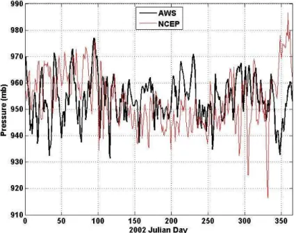
We compared trends in barometric pressure between the two datasets because this is our best indicator as to whether the NCEP/NCAR reanalysis synoptic weather is actually being felt at the lake. The cross correlation coefficient over the entire record

5

between the two was 0.92, which indicates that the NNR model is likely capturing the synoptic scale weather trends experienced at the lake, though there was a mean difference between the two of about 61 mb. This difference is likely caused mainly by the coarse topography used in the NNR model. Comparison of daily values shows that trends are largely being captured (Fig. 7), though it seems that NNR has difficulty

10

capturing large drops in pressure. This discrepancy may also be due to the coarse NNR topography not capturing the confined bowl shape of the basin that could lead to accumulations of cold dense air, since spring and fall showed the best match of magnitudes with winters the worst. However, it is clear from the figure that when a sudden drop or rise is not captured by NCEP/NCAR reanalysis, the subsequent daily

15

values show their worst correspondence in terms of magnitude. However, as the high cross-correlation coefficient indicates, the subsequent trends still track well despite the offset in values, and it is these trends that we are most interested in.

4 Trends in NCEP air temperature and precipitation

Figure 5 shows a striking warming trend in NCEP/NCAR reanalysis MAAT beginning

20

about 1988. From 1960 to 1988, the mean NNR MAAT was ₋12.1◦C with a stan-dard deviation of 0.79◦_{C and a slight cooling trend. From 1989 to 2009, the mean}

MAAT was₋10.1◦C more than 2 standard deviations higher than the previous period. Prior research here (Nolan and Brigham-Grette, 2007) noted the start of this trend (up to 2002) and attributed it to winter warming, with negative degree day (NDD) rising

25

(12)

CPD

8, 1443–1483, 2012

M. Nolan

Title Page

Tables Figures

◭ ◮

Back Close

Full Screen / Esc

Discussion

P

a

per

|

Dis

cussion

P

a

per

|

Discussion

P

a

per

|

Discussio

n

P

a

per

in the number of days below₋30◦_{C. That is, all of this warming could be explained by}

changing in winter temperatures. We can further confirm the general conclusion that winters show more variability now using our AWS data from 2002–2007, which shows a great correspondence with NCEP/NCAR reanalysis in PDD in terms of magnitude and variability and a similarly large variation in NDD (Fig. 5). However, the NDD

mag-5

nitudes themselves do not match as closely between datasets as PDD, and our AWS record is not long enough to confirm the timing and magnitude of the winter warm-ing indicated by the reanalysis data. Thus it appears that in the modern environment that winter temperatures show the most variability. Therefore one of our main goals in our companion paper (Nolan et al., 2012) is to use the SOM method to determine

10

which weather patterns are most responsible for winter warm temperature anomalies and then determine whether this recent warming trend was caused by an increase in frequency of these patterns or whether these patterns change in thermodynamics by transporting warmer air. In this paper, of most relevance is that summer temperatures show little variability over the past 50 years and that the NCEP trend captures summer

15

magnitude well, which we argue later leaves little possibility for multi-year ice cover during this time period.

The length of the summer thaw season is also an important variable affecting many proxy dynamics, so we used the NCEP/NCAR reanalysis record to reconstruct this for the modern period. Given that individual years are often noisy around the spring and

20

fall transitions around zero degrees, we fitted a sinusoid through each year individually and used the zero degree crossing points of this sinusoid to define season length. Manual inspection of each year’s fit showed this to be a reliable technique. The results are plotted in Fig. 8a and b. In Fig. 8a, we show the actual zero-crossing dates and draw a vertical bar between them to indicate the thaw season. The mean start and end

25

(13)

CPD

8, 1443–1483, 2012

M. Nolan

Title Page

Tables Figures

◭ ◮

Back Close

Full Screen / Esc

Discussion

P

a

per

|

Dis

cussion

P

a

per

|

Discussion

P

a

per

|

Discussio

n

P

a

per

an increase in means before and after 2000 of nearly 3 weeks. During this time, the change in positive degree days in summer did not show a corresponding trend (Fig. 5), indicating that while summers are getting longer they are not getting hotter. This points towards changes in weather during spring and fall, rather than winter or summer, as being the cause, and we investigate this further in our companion paper (Nolan et al.,

5

2012).

The NCEP/NCAR reanalysis data also shows an increasing trend in precipitation totals over the past 20 years, similar to air temperature (Fig. 9). As can be seen, total precipitation rose about 50 %, from about 35 cm a−1 to about 55 cm a−1. Unlike air temperatures, however, there is no clear cut seasonal explanation – both summer

10

and winter precipitation rose in roughly equal amounts with roughly the same inter-annual trends. Here we have defined the summer period as Day 150–275 based on our AWS tipping bucket, as previously described. The NNR data show that summer precipitation is slightly higher in annual percentage (57 %) than winter. However, based on our previous analysis we know that NNR is overestimating summer rain by 2–4 times

15

measured, but winter NNR values are approximately what we have measured as end of winter snow water equivalent in 1998, 2003, and 2009 and what we measured from lake pressure changes (15.0 cm) in 2002–2003 (Nolan and Brigham-Grette, 2007). So it is likely that winter and summer precipitation rates are roughly equal, or that winter may be a bit higher, but we do not have enough information to support this further. Because

20

we have shown that NCEP/NCAR reanalysis does seem to pick out large inter-annual differences, we suspect that the trends seen in Fig. 9 are likely real, though the values themselves may be off in magnitude. The importance of these trends to the paleo-climate project relate to snow blocking sunlight to the lake water thereby inhibiting photosynethic activity, and rainfall places limits on whether the lake may have dried out

25

(14)

CPD

8, 1443–1483, 2012

M. Nolan

Title Page

Tables Figures

◭ ◮

Back Close

Full Screen / Esc

Discussion

P

a

per

|

Dis

cussion

P

a

per

|

Discussion

P

a

per

|

Discussio

n

P

a

per

capturing the full range of modern variability here, and even the wettest years are still pretty dry.

5 Use of NCEP/NCAR reanalysis trends to predict lake-ice and lake water-level dynamics

Analysis of paleoclimate proxies thus far has indicated that lake ice cover may have

5

been permanent for periods of thousands of years, exerting strong controls on lake biogeochemistry and creating a need to understand lake ice dynamics better. Nolan et al. (2003) analyzed modern lake ice cover in detail using SAR and Landsat remote sensing as well as numerical models. Here we want to extend these results to the NCEP/NCAR reanalysis time period and use this analysis to further quantitatively and

10

qualitatively describe the environmental conditions necessary for permanent ice cover. We do this, in part, by introducing a simple numerical model that can be used as a starting point by paleo-climatologists later to help constrain individual proxy interpreta-tions.

Ice growth on arctic lakes and rivers can be modeled reasonably successfully

us-15

ing freezing degree days and local tuning factor (USACE, 2004; Arp et al., 2010), in a much simpler way than our prior methods (Nolan et al., 2003). The model we use here (Eq. 1) is a simplified empirical form of the Stefan equation as derived in US-ACE (2002) along with related assumptions and simplifications. In short it assumes vertical, one-dimensional, quasi-steady heat conduction through a uniform, horizontal

20

ice layer, which is only growing at the ice-water interface.

Z_growth₌α′

∗√NDD, (1)

where NDD are negative degree days (expressed as a positive number) in◦_C,_Z growth

is in centimeters, and α′ becomes a local tuning factor, though it has more physical meaning in the full differential equations (USACE, 2002).

(15)

CPD

8, 1443–1483, 2012

M. Nolan

Title Page

Tables Figures

◭ ◮

Back Close

Full Screen / Esc

Discussion

P

a

per

|

Dis

cussion

P

a

per

|

Discussion

P

a

per

|

Discussio

n

P

a

per

Prior research has shown that the differences between this model and more sophis-ticated ones are small, usually less than 15 cm at the end of winter, largely because the simplified model is easily tuned to match, especially in static growth conditions like lakes with no river flux, and is a standard method in ice engineering (Ashton, 1986; US-ACE, 2002). In all models, as the ice gets thicker, it insulates more and slows growth

5

at the lower interface, and this dynamic seems to be the most important one to match. The addition of snow slows heat transfer further. Because the ice grows fastest when it is thinnest, all else equal, the timing of snowfall (and its insulating value) can strongly affect growth, especially in the early season. However, Eq. (1) does not account for inter-annual changes in snowpack (as did our prior model), but rather parameterizes

10

nearly all local e_ffects in the tuning coe_fficientα′, and therefore all conclusions below are based on snowpack dynamics remaining constant through time.

The equation can be used to track growth using NDD accumulating as a function of time or simply calculate final ice thickness using the annual accumulated NDD. Values forα′vary in the literature as this is a site dependent tuning parameter; we used 2.8 to

15

match the maximum 1999–2000 ice thickness of 1.85 m using NCEP/NCAR reanalysis air temperature, assuming that freezing did not begin until₋400 degree days had accu-mulated in fall. This value of₋400 was calculated based on freeze-up not starting until about 18 October, based on several years of remote sensing data (Nolan et al., 2003). A number of factors lead to the formation of ice as described nicely by Locke (1990),

20

but typically sub-freezing temperatures, cold skies, and calm winds are required to ini-tiate a stable ice cover. The ice must then grow thick enough to prevent wind action from starting the process over. We noticed ice skims forming in August 2000 on calm clear nights at Lake El’gygytgyn, but wave action quickly destroyed them the next day. By mid-October air temperatures are cold enough that ice is growing at over 5 cm per

25

day once nucleated and wind can no longer mechanically break the pack completely after a day or two of such growth as leads quickly skim over in the cold temperatures.

(16)

CPD

8, 1443–1483, 2012

M. Nolan

Title Page

Tables Figures

◭ ◮

Back Close

Full Screen / Esc

Discussion

P

a

per

|

Dis

cussion

P

a

per

|

Discussion

P

a

per

|

Discussio

n

P

a

per

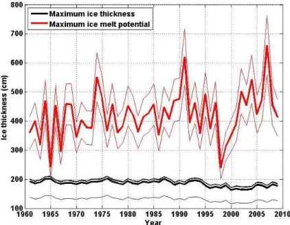
sensitivity of our choice of α′ and freeze-up lag. Figure 10 (thick black line) shows end of winter ice thickness maximums based on the mean daily NCEP/NCAR reanal-ysis air temperatures over the full record (Fig. 2). As can be seen, the recent winter warming reduces ice thickness by 10–30 cm. Here it should be noted that we used NDD calculated from a calendar year (that is, January–May and October–December of

5

the same year) rather than the prior winter (October–May), largely for numerical con-venience, but we spot checked this to find little difference and it is clear that over the full time period that the variability in ice thickness predicted by this crude technique is small, 190 cm_±15 cm. We tested the sensitivity of our methods by eliminating the 400 degree day freeze-up lag (essentially assuming there was no wind and that ice

10

forms as soon as air temperatures drop below zero) and found that this resulted only in about 10 cm of increased thickness (Figure 10, thin black line above thick one). Our value forα′was the highest we found in the literature; using the lowest value we found, 1.7, maximum ice thickness decreased by about 50 cm (Fig. 10, thin black line below thick one). Thus we believe this model and our methods are reasonably robust and the

15

results reliable for our purposes within several decimeters.

In terms of initiating and maintaining a multi-year ice cover, predicting how ice grows is not as important as predicting how lake ice melts, and this unfortunately is a much more complicated process as it is more site dependent. Our prior remote sensing from 1997–2001 indicates that snow melt on the lake surface begins in mid-May, a

20

moat forms at the edge of the lake ice in the last week of June, and complete ice melt occurs in mid-July. Once the moat opens up in June, the ice pack is subjected to substantially higher mechanical erosion due to wind shove, and our remote sensing data show (Nolan et al., 2003) that soon after moat formation, the ice pack forms major leads across the lake at deltas or outcrops which jut into the lake (e.g. at Stream

25

(17)

CPD

8, 1443–1483, 2012

M. Nolan

Title Page

Tables Figures

◭ ◮

Back Close

Full Screen / Esc

Discussion

P

a

per

|

Dis

cussion

P

a

per

|

Discussion

P

a

per

|

Discussio

n

P

a

per

side of the lake to the other based on wind direction, causing massive ground-shove features as it becomes grounded (e.g. Fig. 1), and turning the pack into a jumble of bits rather than cohesive floes. The ice typically disappears completely within a few days of separate floes forming, given the nearly constant wind.

Thus there are at least three important variables in predicting ice cover loss in

sum-5

mer here – simple ice melt from summer sun and warm air, moat formation, and wind action. Unfortunately physically modeling moat formation requires a full 3-D model with more input data than we have. The modern moat is likely formed by a combina-tion of snow meltwater accumulacombina-tion from the ice surface and surrounding landscape plus, and perhaps more importantly, from solar heating of the shallow shelves (<5 m

10

deep) which warm considerably from solar inputs through the snow-free lake ice. Our thermistor string measurements show that water here can reach 5◦C in spring. The shelves are likely former beaches, formed when the lake level was lower (Juschus et al., 2011). If lake water levels were 20 m lower than currently, the area of lake bed that could absorb significant solar radiation (the littoral zone) would be minimal, as

15

it would be confined to a narrow strip of the sides of the steeply sloping bed (10◦–40◦ slope), and all of the water-warming found today in the substantial lagoons and shelves would likely not occur. Thus in glacial times, when precipitation inputs were likely much lower due to the global ice sheet dominance, moats might have been much smaller and harder to form. Without moats, mechanical erosion caused by wind would also

20

have to have been smaller, and the effect of wind itself would have decreased as the lake surface would be more deeply recessed into the lake basin itself. Again these are affects beyond the scope of this paper to try to quantify, but we believe it reasonable to assume that lower lake levels would promote multi-year ice formation, all else being equal.

25

(18)

CPD

8, 1443–1483, 2012

M. Nolan

Title Page

Tables Figures

◭ ◮

Back Close

Full Screen / Esc

Discussion

P

a

per

|

Dis

cussion

P

a

per

|

Discussion

P

a

per

|

Discussio

n

P

a

per

driving fields and found that melting a 1.8 m ice pack takes about 4 weeks by simple melt alone, starting when air temperature rose above freezing and ending at about the summer peak in temperatures (12–15◦C). This model also ignores the all 2-3-D effects, such as melting at grain boundaries causing candle ice formation and the influence of moats and wind. However, the predicted ice-out date due to 1-D melt alone was within

5

a few days of actual, so we conclude that degree days are a reasonable proxy for the combined actions of all influences. In this paper we use positive degree days corrected by a local tuning factor following Bilello (1964):

Z_melt₌Z_max₋α′′

∗PDD, (2)

where Zmax is the end of winter maximum ice thickness,α′′is a tuning factor, and PDD

10

are positive degree days. Values forα′′vary in the literature from 0.2 to 2.0; we used 0.65 to match our 1999–2000 melt curve. Like Eq. (1), Eq. (2) can be used to track melt using PDD as a function of time. The melt curve can be truncated as zero ice thickness, or the second term in Eq. (2) can be used alone with the maximum PDD to calculate ice melt potential, meaning the maximum amount of ice that could be melted

15

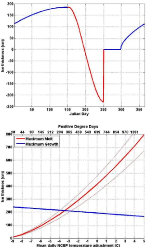
had it been present at end of winter. Figure 11a demonstrates use of these equations graphically.

We used this model to calculate ice melt potential for the NCEP/NCAR reanalysis record in Fig. 10, which revealed that modern summers can melt twice as much ice as is actually formed in modern winters. Here we began accumulating PDD once the

20

smoothed air temperatures rose above zero, as described previously, with no lag. Of particular note is that the variability in potential ice melt is much higher than the variabil-ity in ice growth and that the magnitude is always much higher. Given that there was little trend in PDD (Fig. 6), it is not surprisingly there is little trend in potential ice melt. Thin red lines in Fig. 10 estimate error based on the range ofα′′from 0.2 to 2.0 found in

25

(19)

CPD

8, 1443–1483, 2012

M. Nolan

Title Page

Tables Figures

◭ ◮

Back Close

Full Screen / Esc

Discussion

P

a

per

|

Dis

cussion

P

a

per

|

Discussion

P

a

per

|

Discussio

n

P

a

per

How much colder does it need to be to maintain a multi-year ice cover? Qualitatively we can see from Fig. 10 that it is summers that need to change the most, but to answer this numerically, we took the mean daily temperatures of the NCEP/NCAR reanalysis record (Fig. 2) and shifted the entire time-series from+5 to₋9◦C. The warmer limit seams reasonable based on climate change scenarios and the colder limit is the point

5

at which there are no longer any positive degree days to promote melt in this model. Figure 11b plots the results of this analysis, which makes it clear that it is really sum-mers that are driving melt, so we also calculated the results in terms of PDD (same curve, top axis). Where the ice growth curve and potential ice melt curve intersect at about₋3.5◦C is what we believe is the minimum MAAT required to initiate a multi-year

10

ice cover. However, given that some ice needs to be left over at the end of summer, we somewhat arbitrarily picked 20 cm as this requirement (which is essentially a tuning factor representing more than just ice thickness), which increases the required MAAT shift to ₋4◦_{C; requiring 50 cm ice remaining at end of summer increases the MAAT}

shift to₋4.5◦C A shift in the mean of ₋4◦C represents a change in PDD from about

15

640 to 280 (Fig. 11b, top x-axis), thus summer needs to be less than half as warm as the modern mean to initiate an perennial ice cover. As length of open water season may be valuable to paleoclimate proxies, we used this model to predict the dates of ice-out, start of ice growth, and start of ice melt in Fig. 12 for the NCEP/NCAR reanalysis record.

20

We further tested the sensitivity of our choice of α′′ by using the maximum range from the literature: a value of 0.2 reduced the potential to about 130 cm and a value of 2.0 increased the potential to about 13 m. Given that these tuning parameters are accounting for all site specific variables (e.g. shading, bathymetry, streamflow, etc.), this range should not be considered real, but it does indicate that our choice of α′′

25

(20)

CPD

8, 1443–1483, 2012

M. Nolan

Title Page

Tables Figures

◭ ◮

Back Close

Full Screen / Esc

Discussion

P

a

per

|

Dis

cussion

P

a

per

|

Discussion

P

a

per

|

Discussio

n

P

a

per

of₋4◦_C

±0.5◦C is a reasonable estimate for initiating a multi-year ice-cover, noting

that this is relative to the NCEP/NCAR reanalysis mean which we know is not a perfect fit to reality but does represent actual summer temperatures well.

While this analysis is crude, it certainly has the right order of magnitude, and given the close correspondence found between model and measurements in previous work,

5

there is good reason to believe that₋4◦C is a reasonable number to initiate a multi-year ice cover. As can be seen from the slope of the lines in Fig. 11b, multi-year ice formation is much more sensitive to summer temperatures than winter temperatures. That is, the range of ice growth under any reasonable modern winter scenario is 1.5 to 2.5 m, but the range of potential ice melt under modern summer scenarios (conservative for

10

paleoclimate) is 3 to 6 m. So even if our ice growth model is not as accurate as we would like to think it is, we know for sure that in postulating colder summers that winters are likely to be colder too, so we know that at least 2 m of ice will form (but probably not a lot more than this in a single year). While determining the tuning factorα′′ for the 2001 melt season data, we found the value could range from 0.55 to 0.75 and still

15

capture the trend, which creates a range of about a week in terms of ice-out date in 2000, and a range of_±0.5◦C in terms of the crossing point in Fig. 11b and is shown on Fig. 10 as thin red lines.

Once a multi-year ice cover forms in glacial times, could ice sublimation rates ex-ceed precipitation inputs and dry out the lake? Unfortunately we do not have enough

20

information in hand about paleo-precipitation except to say at times that it could have been less than today, and while sublimation rates can be calculated by a variety of models of varying sophistication, given our lack of input data any model results would have to be used with great caution. What we do know is that most of the sublimation at the permanently ice-covered lakes in the Dry Valleys of Antarctica occurs during

25

(21)

CPD

8, 1443–1483, 2012

M. Nolan

Title Page

Tables Figures

◭ ◮

Back Close

Full Screen / Esc

Discussion

P

a

per

|

Dis

cussion

P

a

per

|

Discussion

P

a

per

|

Discussio

n

P

a

per

El’gygytgyn were likely warmer during glacial times than modern Dry Valley summers, it seems reasonable to assume that similar rates of summer sublimation might have occurred there too. These ablation rates in Antarctica range from 10 cm to 1.5 m (in-cluding sublimation and evaporation of landlocked melt) with 35 cm per year (Clow et al., 1988; Squyres et al., 1991; Doran et al., 1994, 1996) being typical, which is roughly

5

the amount of modern precipitation at Lake El’gygytgyn. Thus if glacial periods were characterized by less precipitation, which seems likely given (1) the drop in sea level and extended distance to moisture sources, (2) the amount of moisture locked up in ice sheets, and (3) the sharply decreased sedimentation rates in the lake, it is certainly conceivable that sublimation rates may have exceeded precipitation rates. If

sublima-10

tion exceeded precipitation by 5 to 50 cm, which is within reason, the lake would have dried out in 3500 to 35 000 years. Given that glacial epochs often last 50 000 years or more, it seems that there may have been multiple opportunities for dry out. However, given the variability in precipitation and temperature, it is also conceivable that a few centuries or even decades of warmer/wetter weather could balance out several

thou-15

sand years of loss, and there seems to be little bathymetric evidence for submerged paleo-shorelines beyond the current shelves. Completely unaccounted for is the pos-sibility of groundwater infiltration from beneath the thick permafrost layer through the talik that likely exists beneath the lake, as has been suggested previously (Nolan et al., 2003), or its variability over 3.6 M years. Therefore while we do not have enough

infor-20

mation to state that the lake dried out and caused temporal gaps in the proxy record, we can state that it is within the realm of possibility and caution paleo-climatologists to be alert to this possibility in their interpretations.

6 Relevance to paleoclimate reconstructions

If the modern climate record can be used to inform us about paleoclimate (at least on

25

(22)

CPD

8, 1443–1483, 2012

M. Nolan

Title Page

Tables Figures

◭ ◮

Back Close

Full Screen / Esc

Discussion

P

a

per

|

Dis

cussion

P

a

per

|

Discussion

P

a

per

|

Discussio

n

P

a

per

of this paper is that winter variability does little to affect the formation of multi-year ice covers. What are required are much colder summers than today, regardless of what happens during winter. We address the synoptic drivers of air temperature in our companion paper (Nolan et al., 2012) along with some speculations as to which weather patterns likely dominated during the colder/warmer periods.

5

Given that glacial periods over the past 3 600 000 years were often 6◦C colder than today (Petit et al., 1999; Lisiecki and Raymo, 2005), we believe we have strong support for the possibility of permanent ice cover persisting at Lake El’gygytgyn for perhaps as much of half of this time, perhaps more, since most of this time was characterized by temperatures at least 3◦C colder than today. All else being equal, if there was a solid

10

ice pack left once air temperatures dropped below freezing in fall, ice growth would begin immediately as wind disruption will be minimized and growth rates will be high in the thinner ice. In this case, by the end of the next winter, the ice could be an additional 20 cm thicker than had growth started in open water, plus the thickness of any remnant summer ice. Thus after a few cold years of>4◦C colder than today, an ice pack of 3 m

15

or more could have formed, which could be maintained through subsequent years of only 2–3◦_{C colder weather (Fig. 11b). Ice growth would eventually reach an equilibrium}

thickness as it does in the Dry Valleys, and not continue to increase with time. Similarly, any number of scenarios can be imagined in which a multi-year ice cover can survive an occasional warm year, much in the way that multi-year sea ice reacts. That is,

20

similar to sea ice, multi-year lake ice is harder to form than it is to maintain. It is beyond the scope of this paper to test these scenarios, and it is our hope that these simple formulas will be put to use by the paleo-climate community as a starting point for more elaborate scenario testing, and perhaps use of a more sophisticated lake ice model. One cautionary note is that our shift of ₋4◦C is based on the 50 years NCEP/NCAR

25

(23)

CPD

8, 1443–1483, 2012

M. Nolan

Title Page

Tables Figures

◭ ◮

Back Close

Full Screen / Esc

Discussion

P

a

per

|

Dis

cussion

P

a

per

|

Discussion

P

a

per

|

Discussio

n

P

a

per

possibility of Lake El’gygytgyn being perennially covered by ice during this time. In any case, we can say with some confidence that it is possible to maintain a multi-year ice cover and still have a wide-variety of Arctic summer scenarios. A 4◦C reduction in the NCEP/NCAR reanalysis mean daily temperatures shows that there would still have been over 2 months of above freezing temperatures and 30 days during the peak

5

with about a 5◦C mean (this can be visualized by shifting the thick black line in Fig. 2b down by 4◦C and seeing what remains above 0◦C). Thus many summer-time biolog-ical processes could still have been active and contributing to the proxy record in the sediment core. The mean would have to be reduced by over 9◦C to completely elim-inate summer (assuming a similar summer-winter change), and based on long-term

10

reconstructions of air temperatures, such cold snap were rare, if ever, over the duration of the El’gygytgyn record (Petit et al., 1999; Lisiecki and Raymo, 2005). Therefore, just because the lake ice can persist through summer does not mean that summers did not exist, the question is more about the degree of summer conditions that existed, and we hope that proxies may be exploited that have temperature thresholds which could

15

further refine our crude modeling.

Similarly, given that a substantial summer might have existed with perennial ice cover, some warming and mixing of sub-ice lake-water likely also occurred. We in-stalled a thermistor string near the center of the lake and later recovered water temper-ature data from 2000–2003; these data are described in detail in (Nolan and

Brigham-20

Grette, 2007), and show that warming and mixing began during ice melt, at least in the upper 30 m. We also found evidence for a low-flow, toroidally shaped current which brought warm, dense water from the shallow shelves to the deepest part of the lake throughout winter, carrying both biota and nutrients (Nolan et al., 2003), and we have no reason to believe that such a flow would not also have existed beneath a perennial

25

(24)

CPD

8, 1443–1483, 2012

M. Nolan

Title Page

Tables Figures

◭ ◮

Back Close

Full Screen / Esc

Discussion

P

a

per

|

Dis

cussion

P

a

per

|

Discussion

P

a

per

|

Discussio

n

P

a

per

An open question which we have not addressed here numerically is how did any sediment reach the lake floor during prolonged periods of multi-ice cover? Our numer-ical results show that it only takes one year of modern temperature to melt the thickest reasonable ice cover (_∼6 m), so it could be that sediment stored in the ice periodically got flushed out. This subject of sediment transport through ice is an active area of

5

research in the lakes of the Dry Valleys (Squyres et al., 1991; Andersen et al., 1993; Doran et al., 1994; Spaulding et al., 1997; Wagner et al., 2006; Jepsen et al., 2010). Here it has been found that surface sediments often found an equilibrium depth (_∼2– 3 m) within the ice and accumulate there. It reaches an equilibrium because as the surface ablates in summer due to sublimation or melt, this loss promotes ice growth

10

from below due to increased heat transport upwards. Thus a competition results from how quickly sediments can melt their way down due to solar gain, compared to how fast the surface melts and bottom grows, among other processes. Significant variation is found lake-to-lake within the Dry Valleys, so no hard conclusions can be drawn for Lake El’gygytgyn. Grain size also seems to matter, as finer particles are able to utilize

15

grain boundaries as conduits. Cracks and leads also serve as fast entry routes. If modern lake levels were maintained in the past, lagoons and moats likely formed and these could have served as quick entry locations at the shoreline for alluvial sediments. If lake levels were more than 10 m lower, it is likely that moats played a smaller role in sediment transport, though possibly still significant. Lake level variations themselves

20

may also have played an important role, as simply raising and lowering the lake ice on decadal-to-millenial scales may have scraped significant amount of shore-accumulated material beneath the ice pack. Similarly, lower lake levels may have led to undercut-ting of fluvial fans, which then either avalanched on to the ice or below it after lake levels rose.

25

(25)

CPD

8, 1443–1483, 2012

M. Nolan

Title Page

Tables Figures

◭ ◮

Back Close

Full Screen / Esc

Discussion

P

a

per

|

Dis

cussion

P

a

per

|

Discussion

P

a

per

|

Discussio

n

P

a

per

sediment free; on a Dry Valley lake, one could likely not slide 10 cm any time of year due to the rough and irregular surface. Perennial ice covers essentially have no choice but to be rougher annual ones because (1) it cannot get any smoother and (2) centuries of differential melt of internal sediments and surface wind scour will certainly beat it up. Because this Antarctic ice surface is so rough and so sediment rich, only a fraction of

5

the sunlight (<3 %) making it through modern Lake El’gygytgyn’s ice makes it through Dry Valley lakes. This likely has important implications for lake biological productiv-ity, and in this regard research from the modern Dry Valleys may serve as a useful analogue to glacial Lake El’gygytgyn.

Acknowledgements. Throughout the paper I have used plural pronoun “we” to describe our

10

efforts, as this research was a team effort; I acknowledge a few key team members here, and also note that any opinions, findings, and conclusions or recommendations expressed in this paper are those of the author and do not necessarily reflect the views of the National Science Foundation, other funding sources, or any of the other team members. I’d like to thank members of the 2000 expedition for helping transport and erect the AWS, including in particular Julie

15

Brigham-Grette and Mike Apfelbaum, and members of the 2009 expedition for downloading the data and dismantling the site, including in particular Volker Wennrich and Julie Brigham-Grette. I would also like to thank Pavel Minyuk for his tireless e_fforts at permitting. Elizabeth and John Cassano provided the NCEP/NCAR reanalysis data and valuable insights into climate models. This work was supported by National Science Foundation Grants OPP 0075122, 96-15768,

20

and 0002643 and EAR 0602512.

References

Andersen, D. W., Wharton, R. A., and Sqryres, S. W.: Terrigenous Clastic Sediments in Antarc-tic Dry Valley Lakes, Antar. Res. Ser., 59, 71–81, 1993.

Arp, C. D., Jones, B. M., Whitman, M., Larsen A., and Urban, F. E.: Lake temperature and ice

25

cover regimes in the Alaskan Subarctic and Arctic: Integrated monitoring, remote sensing, and modeling, J. Am. Water Resour. As., 46, 777–791, 2010.

Ashton, G. D.: River and lake ice engineering. Littleton, CO, Water Resources Publica-tions, 1986.

Belya, B. and Chershnev, I. A.: The nature of the El’gygytgyn Lake Hollow, Magadan, Russian

30

(26)

CPD

8, 1443–1483, 2012

M. Nolan

Title Page

Tables Figures

◭ ◮

Back Close

Full Screen / Esc

Discussion

P

a

per

|

Dis

cussion

P

a

per

|

Discussion

P

a

per

|

Discussio

n

P

a

per

Bilello, M.: Method for predicting river and lake ice formation, J. Appl. Meteorol., 3, 38– 44, 1964.

Brigham-Grette, J.: Contemporary Arctic change: A paleoclimate d `eja‘ vu?, Proc. Natl. Acad. Sci., 44, 18431–18432, 2009.

Brigham-Grette, J., Melles, M., Minyuk, P., and Party, S.: Overview and significance of a 250

5

ka paleoclimate record from El’gygytgyn Crater Lake, NE Russia, J. Paleolimnol., 37, 1– 16, 2007.

Brigham-Grette, J., Melles, M., and Minyuk, P.: Climate variability from the Peak Warmth of the Mid-Plicene to Early Pleistocene from Lake El’gygytgyn northerstern Russia, western Beringia, Climate of the Past, this issue, in prep., 2012.

10

Cherapanova, M. V., Snyder, J. A., and Brigham-Grette, J.: Diatom stratigraphy of the last 250 ka at Lake El’gygytgyn, northeast Siberia, J. Paleolimnol., 37, 155–162, 2007.

Clow, G., McKay, C., Simmons, G., and Wharton Jr., R.: Climatological observations and pre-dicted sublimation rates at Lake Hoare, Antarctica, J. Climate, 1, 715–728, 1988.

Cremer, H. and Wagner, B.: The diatom flora in the ultra-oligotrophic Lake El’gygytgyn,

15

Chukotka, Polar Biology, 26, 105–114, 2003.

DeConto, R. and Koenig, S.: Responseof western Beringian climte due to Plio-Plesitocene climate forcings, Climate of the Past this issue, in prep., 2012.

Doran, P. T., Wharton, R. A., and Lyons, W. B.: Paleolimnology of the McMurdo Dry Valleys, Antarctica, J. Paleolimnol., 10, 85–114, 1994.

20

Doran, P. T., McKay, C., Meyer, M. A., Andersen, D. T., Wharton Jr., R., and Hastings, J. T.: Climatology and implications for perennial lke ice occurrence at Bunger Hills Oasis, East Antarctica, Antarct. Sci., 8, 289–296, 1996.

Federov, G., Nolan, M., Brigham-Grette, J., Bolshiyanov, D., Schwamborn, G., and Juschus, O.: Lake El’gygytgyn water and sediment balance components overview and its implications

25

for the sedimentary record, Climate of the Past, this issue, in prep., 2012.

Glushkova, O.: Geomorphology and history of relief development of El’gygytgyn Lake Region, in: The nature of the El’gygytgyn Lake Hollow, edited by: Belya, V. F. and Chershnev, I. A., Magadan, Russian Academy of Science, 26–48, 1993.

Glushkova, O. Y. and Smirnov, V. N.: Pliocene to Holocene geomorphic evolution and

paleo-30

geography of the El’gygytgyn Lake region, NE Russia, J. Paleolimnol., 37, 37–47, 2007. Jepsen, S., Adams, E., and Priscu, J.: Sediment melt-migration dynamics in perennial Antarctic

(27)

CPD

8, 1443–1483, 2012

M. Nolan

Title Page

Tables Figures

◭ ◮

Back Close

Full Screen / Esc

Discussion

P

a

per

|

Dis

cussion

P

a

per

|

Discussion

P

a

per

|

Discussio

n

P

a

per

Juschus, O., Pavlov, M., Schwamborn, G., Federov, G., and Melles, M.: Lake Quarternary lake-level changes of Lake El’gygytgyn, NE Siberia, Quarternary Res., 76, 441–451, 2011. Kalnay, E., Kanamitsu, M., Kistler, R., Collins, W., Deaven, D., Gandin, L., Iredell, M., Saha,

S., White, G., Woollen, J., Zhu, Y., Leetmaa, A., Reynolds, B., Chelliah, M., Ebisuzaki, W., Higgins, W., Janowiak, J., Mo, K. C., Ropelewski, C., Wang, J., Jenne, Roy, and Joseph, 25

5

Dennis: The NCEP/NCAR 40 year reanalysis project, B. Am. Meteorol. Soc., 77, 437–471, 1996.

Kane, D. L. and Yang, D.: Northern Research Basins Water Balance, International Association Hydrological Sciences Publication, 290, 271 pp., 2004.

Kaufman, D. S., Schneider, D. P., McKay, N. P., Ammann, C. M., Bradley, R. S., Briffa, K. R.,

10

Miller, G. H., Otto-Bliesner, B. L., Overpeck, J. T., Vinther, B. M., and Arctic Lakes 2k Project Members: Recent Warming Reverses Long-Term Arctic Cooling, Science, 325, 1236–1239, 2009.

Layer, P.: Argon-40/Argon-39 age of the El’gygytgyn impact event, Chukotka, Russia, Meteorit. Planet. Sci., 35, 591–599, 2000.

15

Lisiecki, L. E. and Raymo, M. E.: A Pliocene-Pleistocene stack of 57 globally distributed benthic δ18O records, Paleoceanography, 20, PA1003, doi:10.1029/2004PA001071, 2005.

Locke, G. S. H.: The growth and decay of ice, Cambridge, Cambridge University Press, 1990. Melles, M., Brigham-Grette, J., Glushkova, O. Y., Minyuk, P. S., Nowaczyk, N. R., and

Hub-berten, H. W.: Sedimentary geochemistry of core PG1351 from Lake El’gygytgyn – a

sen-20

sitive record of climate variability in the East Siberian Arctic during the past three glacial-interglacial cycles, J. Paleolimnol., 37, 89–104, 2007.

Melles, M., Brigham-Grette, J., and Minyuk, P.: Evolution of Quarternary Arctic climate from Lake El’gygytgyn, northeastern Russia, Climate of the Past, this issue, in prep., 2012. Minyuk, P. S., Brigham-Grette, J., Melles, M., Borkhodoev, V. Y., and Glushkova, O. Y.: Inorganic

25

geochemistry of El’gygytgyn Lake sediments northeastern Russia as an indicator of paleocli-matic change for the last 250 kyr, J. Paleolimnol., 37, 123–133, 2007.

Minyuk, P., Borkodoev, V., and Wennrich, V.: Inorganic data from El’gygytgyn Lake sediments 1: Marine isotope stages 6–11, Climate of the Past, this issue, in prep., 2012.

Nolan, M. and Brigham-Grette, J.: Basic hydrology, limnology, and meteorology of modern Lake

30

El’gygytgyn, Siberia, J. Paleolimnol., 37, 17–35, 2007.