Short Report
S
J. Braz. Chem. Soc., Vol. 22, No. 11, 2225-2233, 2011.Printed in Brazil - ©2011 Sociedade Brasileira de Química 0103 - 5053 $6.00+0.00
*e-mail: [email protected]
Effect of the Subsampling Ratio in the Application of Subagging for Multivariate
Calibration with the Successive Projections Algorithm
Arlindo R. Galvão Filho,a Roberto K. H. Galvãoa and Mário César U. Araújo*,b
aInstituto Tecnológico de Aeronáutica, Divisão de Engenharia Eletrônica,
12228-900 São José dos Campos-SP, Brazil
bUniversidade Federal da Paraíba, CCEN, Departamento de Química,
CP 5093, 58051-970 João Pessoa-PB, Brazil
Este artigo estuda o efeito da razão de subamostragem na abordagem subagging para regressão linear múltipla com seleção de variáveis pelo algoritmo das projeções sucessivas. Para isso, apresentam-se investigações envolvendo dados simulados e também determinação de umidade e proteína em trigo e temperaturas de destilação (T10 e T90), massa específica e enxofre em diesel por espectrometria no infravermelho próximo. Em termos de capacidade de predição e sensibilidade a ruído, os melhores resultados foram obtidos para razões de subamostragem em torno de 40%.
This paper concerns the effect of the subsampling ratio on the subagging approach for multiple linear regression with variable selection by the successive projections algorithm. Investigations involving simulated data, as well as near-infrared spectrometric determination of moisture and protein in wheat and distillation temperatures (T10 and T90), specific mass and sulphur in diesel, are presented. In terms of prediction ability and sensitivity to noise, the best results were obtained for subsampling ratios around 40%.
Keywords: multivariate calibration, successive projections algorithm, subagging, near-infrared spectrometry, wheat, diesel
Introduction
The successive projections algorithm (SPA)1 was
developed to select subsets of variables with small multi-collinearity for use in multiple linear regression (MLR) models. MLR-SPA has been employed, for example, in spectrometric determination of solubility of solids in
beers,2 glucose in human blood,3 quality parameters of
vegetable oils,4 phenolic compounds in sea water,5 sulphur
in diesel,6 and various other applications. A graphic
user interface for MLR-SPA is publicly available at http://www.ele.ita.br/~kawakami/spa.
In addition to new analytical applications of MLR-SPA, several works have also been conducted on the implementation aspects of the algorithm itself. Gains in parsimony were achieved, for example, by identifying variables that can be removed from the model without
compromising its prediction ability.7 Improvements
were also obtained by exploiting the correlation with the
dependent variable in the projections phase of MLR-SPA.8
More recently, a modification was proposed to deal with the presence of unknown interferents in the samples to be
analyzed.9 Improvements concerning computational issues
have also been reported.10,11
In this context, it has been shown12 that MLR-SPA
results can be improved by using a statistical technique called subagging (subsample aggregating). Such a technique consists of combining different models obtained as the result of a process of subsampling.13 In the
MLR-SPA-subagging case, the subsampling procedure can be regarded as a random splitting of the modelling data into calibration and validation sets. In a subsequent work, this approach was adapted for use in a calibration transfer
framework.14 For this purpose, transfer samples were
inserted in the validation set formed at each subsampling iteration.
An important factor, which was not addressed in
the previous MLR-SPA-subagging works,12,14 concerns
In both investigations,12,14 this ratio was arbitrarily set to
approximately 60% (number of calibration samples/number of calibration plus validation samples). The present paper investigates the effect of the subsampling ratio on the resulting MLR-SPA-subagging model. For this purpose, case studies involving simulated data, as well as near-infrared (NIR) spectrometric determination of moisture and protein in wheat and T10, T90, specific mass and sulphur in diesel are presented. The results are evaluated in terms of the prediction ability and sensitivity to spectral measurement noise.
Background and theory
MLR-SPA
In the original implementation of MLR-SPA,1 it is
assumed that the Nmod samples available for modelling
purposes have been divided into a calibration and a
validation sets, with Ncal and Nval samples, respectively
(where Nmod = Ncal + Nval). The instrumental response
data of the calibration set are then arranged in a matrix
Xcal (Ncal × K) where Ncal and K denote the number of
samples and variables, respectively. A series of projection
operations involving the columns of matrix Xcal is then
employed to form K chains with M variables each, where M = min(Ncal − 1, K). The first element of the kth chain
corresponds to variable xk. Each subsequent element in the
chain is selected in order to display the least collinearity with the previous ones. Subsets of variables extracted from the chains are then evaluated on the basis of the prediction ability of the resulting MLR models in the validation set. The best subset of variables is then chosen according to a suitable performance criterion, such as the root-mean-square error of validation. Finally, a statistical hypothesis test is employed to remove variables from this subset without compromising the prediction ability of the
MLR model.7
MLR-SPA-subagging
The MLR-SPA outcome depends on the choice of calibration and validation sets from the available samples.
In the MLR-SPA-subagging approach,12 this aspect is
exploited to generate a pool of different MLR models which are then aggregated into an ensemble model. Each individual model is obtained by randomly splitting the modelling samples into calibration and validation sets and then applying MLR-SPA. At the end, model aggregation is carried out by co-averaging the individual model predictions as
(1)
where ŷav and ŷ(n) denotes the predictions of the ensemble
model and the nth individual model, respectively. In
what follows, the number of subsampling iterations (i.e.,
the number of aggregated models) will be denoted by
P, as in equation 1. Typically, it has been found12 that
the MLR-SPA-subagging procedure tends to converge after the aggregation of approximately P = 30 individual models.
It is worth noting that the co-averaging procedure expressed in equation 1 can also be reformulated in terms
of the regression coefficients of the MLR models, i.e.,
(2)
(3)
where
(4)
If a certain variable xk was not selected by MLR-SPA
for inclusion in a particular individual model, the
corresponding regression coefficient bk is set to zero in
that model. For example, assume that K = 3 variables are available for selection and that P = 2 individual models are obtained in the MLR-SPA-subagging procedure. Furthermore, suppose that variables x1 and x3 are selected
in the first MLR-SPA model and variables x2 and x3 are
selected in the second MLR-SPA model. In this case, these models could be expressed as
(5)
(6)
Equations 5 and 6 can be rewritten as
(7)
(8)
where a null regression coefficient was assigned to variables x2 and x1 in the first and second models, respectively. The
coaveraging procedure can then be employed as in equation 4 with b2
(1) = 0 and b 1 (2) = 0.
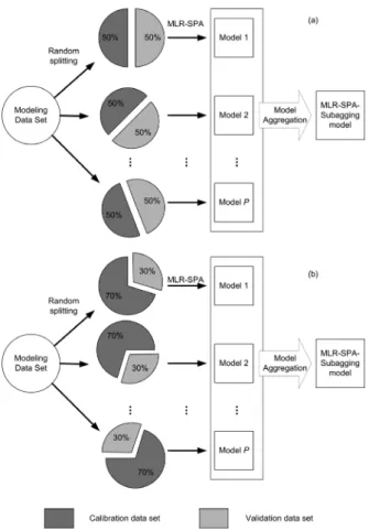
Within this context, an important design parameter is the subsampling ratio q defined as
For illustration, Figure 1 depicts the MLR-SPA-subagging procedure for two different subsampling ratios, namely q = 50% (Figure 1a) and q = 70% (Figure 1b).
As mentioned above, in previous works concerning the
use of MLR-SPA-subagging,12,14 the subsampling ratio q
was arbitrarily set to approximately 60%. However, it may be argued that better ensemble models could be obtained by
using a different choice for q, which motivates the present investigation.
Experimental
Simulated data set
Simulated spectra were generated as in a previous work
involving MLR-SPA.7 For this purpose, a linear relation was
assumed between the matrix X of instrumental responses and the matrix Y of analyte concentrations:
X = YW + N (10)
where N is a noise term. Three analytes (termed A, B,
and C) and K = 300 spectral variables were considered. Matrix W (3 × 300) contains the proportionality coefficients between the analyte concentrations and the instrumental responses. The W-values adopted in this simulated study are presented in Figure 2a.
A total of 200 spectra were generated by using a matrix
Y (200 × 3) with concentration values randomly distributed
in the range 1-10 (arbitrary units). Gaussian noise with zero mean and standard deviation of 0.1 was added to all spectra as in equation 10. The resulting spectra are presented in Figure 2b.
The overall set of Ntot = 200 spectra was divided into
a modelling set with Nmod = 100 samples and a prediction
set with Npred = 100 samples (Ntot = Nmod + Npred) by
applying the Kennard-Stone (KS) algorithm19 to the matrix
X (200 × 300) of instrumental responses. The modelling
set was employed in the MLR-SPA-subagging procedure, as described in the previous section. The prediction set was only employed to evaluate and compare the performance of the resulting models.
Figure 1. MLR-SPA-subagging procedure for (a) q = 50% and (b) q = 70%.
Wheat data set
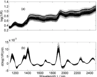
This public data set consists of NIR diffuse reflectance
spectra of Ntot = 100 wheat samples, along with reference
values of moisture and protein content.15,16 The spectra were
acquired in the range 1100-2500 nm with a 2 nm resolution, resulting in 701 spectral variables.
Figure 3 shows the NIR spectra of the 100 wheat samples. As can be seen in Figure 3a, the spectra display baseline shifts, which were eliminated by using
a first-derivative Savitzky-Golay filter with a 2nd-degree
polynomial and a 21-point window.17 The resulting
derivative spectra are shown in Figure 3b. Finally, the number of variables was reduced by discarding those for which the maximum signal intensity over all derivative spectra did not exceed 2% of the maximum signal intensity
in the overall data set.18 The resulting spectra comprised
K = 652 variables.
The overall set of Ntot = 100 wheat samples was divided
into a modelling set with Nmod = 70 samples and a prediction
set with Npred= 30 samples (Ntot = Nmod + Npred) by applying the KS algorithm to the matrix X (100 × 652) of derivative spectra.
Diesel data set
This data set, which comprises 170 diesel samples collected from gas stations in the city of Recife (Pernambuco State, Brazil), was employed in a previous MLR-SPA-subagging study.12 The reference values for sulphur content,
specific mass, and distillation temperatures (T10 and T90) were obtained according to the ASTM (American Society for Testing and Materials) D4294-90, 4615, and D86 methods, respectively. NIR spectra in the range 885-1600 nm were acquired using a FT-NIR/MIR spectrometer Perkin Elmer
GX with an optical path length of 1.0 cm and a spectral
resolution of 2 cm-1. Systematic variations in the baseline
were circumvented by using derivative spectra calculated with a Savitzky-Golay filter (2nd-order polynomial, 11-point
window). As a result, the number of spectral variables was K = 1431. The original and derivative NIR spectra of the 170 diesel samples are presented in Figures 4a and 4b, respectively.
The overall set of Ntot = 170 diesel samples was divided into a modelling set with Nmod = 85 samples and a prediction
set with Npred = 85 samples (Ntot = Nmod + Npred) by applying the KS algorithm to the matrix X (170 × 1431) of derivative
spectra.
Evaluation of the MLR-SPA-subagging models
The MLR-SPA-subagging models were obtained for nine different subsampling ratios, namely q = 10%, 20%, ..., 90%. It is worth noting that such percentages are expressed in terms of the Nmod modelling samples, as indicated in equation 9. In
each case, the ensemble models were evaluated in terms of predictive ability and sensitivity to instrumental noise. The predictive ability was assessed by calculating the root-mean-square error in the prediction set (RMSEP) as
(11)
where yi and ŷi are the reference and the predicted values
of the property under consideration for the ith prediction sample.
Sensitivity to instrumental noise was taken into account as suggested elsewhere20-22 by calculating the 2-norm of the
regression vector (||bav||), which is defined as:
Figure 3. (a) Original and (b) derivative spectra of the wheat samples.
(12)
where bkav denotes the regression coefficient associated to
variable xk in the ensemble model. In fact, by following the
demonstration provided by Pinto et al.,20 it can be shown
that σŷav = σnoise ||bav||, where σnoise is the standard deviation of the instrumental noise (assumed to be homoscedastic
and uncorrelated across the model variables) and σŷav
is the standard deviation of the error in the ensemble model predictions resulting from the propagation of the instrumental noise. Ideally, improvements in the ensemble
model should provide reductions in both RMSEP and ||bav||.
It is worth noting that MLR-SPA-subagging has a stochastic nature due to the random subsampling operations. Therefore, given a certain subsampling ratio q and number of iterations P, the RMSEP and ||bav|| values may
vary for different realizations of the MLR-SPA-subagging procedure. For this reason, in order to assess the dispersion
of the results, a Monte Carlo simulation23 was carried out by
calculating the average and standard deviation of the results
over several realizations. In the present work, nMC = 25
realizations were employed in the Monte Carlo simulation.
Software
All calculations were carried out using the Matlab 2009b software. The subsampling operations in the MLR-SPA-subagging procedure were performed by using random permutations with the “rand” Matlab routine.
Results and Discussion
Simulated data set
Figure 5 presents the results obtained for analytes A and B with a fixed subsampling ratio (q = 70%) and a number of iterations P ranging from 1 to 50. The results for analyte
Figure 5. MLR-SPA-subagging results as a function of the number of iterations: RMSEP for (a) analyte A and (b) analyte B, ||bav|| for (c) analyte A and
C were similar to those obtained for analyte A and are thus omitted for brevity. As can be seen, there is a marked
improvement in RMSEP and ||bav|| for both analytes as the
number of iterations P is increased. However, the gains become marginal after P = 30, which is in agreement with
the findings reported elsewhere.12
The average results obtained for different subsampling ratios are shown in Figure 6. In this case, the number of iterations was set to P = 30, because the improvements for more iterations were marginal as discussed above. The
error bars for RMSEP and ||bav|| correspond to standard
errors, which were calculated as the standard deviation σ
divided by the square root of the number of Monte Carlo
realizations nMC (i.e., ).
In the ||bav|| × RMSEP plots presented in Figure 6, the best
results are those situated closest to the origin (small values for both ||bav|| and RMSEP). In this sense, Figure 6a indicates that
appropriate subsampling ratios for determination of analyte A range from 20% to 40%. Within this range, the changes in ||bav|| are minor and the difference between the smallest and
largest RMSEP values are not significant according to an
F-test at 95% confidence level. Other values for q (10% and
50-90%) lead to an increase in both ||bav|| and RMSEP. The
same comments regarding the choice of q can be applied to analyte B (Figure 6b). It is worth noting that the RMSEP and ||bav|| results are generally worse for analyte B as compared
to analyte A. Such a finding can be ascribed to the fact that the spectrum of analyte B is strongly overlapped by the two other analytes (A and C, as seen in Figure 2a).
Wheat data set
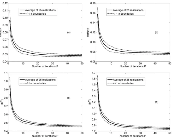
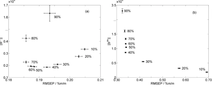
Figure 7 presents the protein and moisture results obtained for a fixed subsampling ratio (q = 70%) and a
number of iterations P ranging from 1 to 50, as in Figure 5. As in the simulated case study, a marked improvement
in RMSEP and ||bav|| for both protein and moisture can
be observed as the number of iterations is increased up to P = 30. In this case, it is worth noting that the results are statistically unstable for P < 10, as indicated by the large standard deviation values at the beginning of the curves.
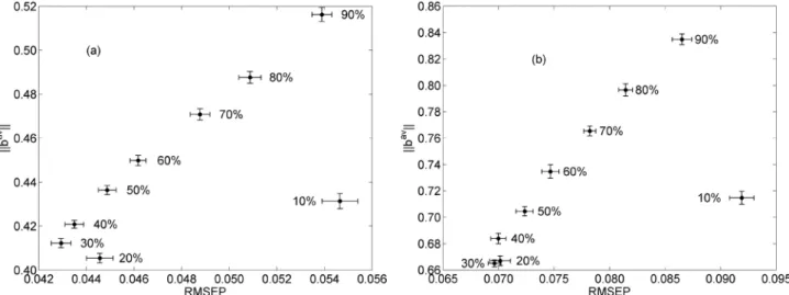
The average results obtained for different subsampling ratios with P = 30 are shown in Figure 8. As can be seen in Figure 8a, appropriate subsampling ratios for moisture determination range from 30 to 70%. Within this range,
the changes in ||bav|| are minor and the difference between
the smallest and largest RMSEP values are not significant
according to an F-test at 95% confidence level. Smaller
values for q (10 and 20%) lead to a noticeable increase in RMSEP, whereas larger values for q (80 and 90%) result in substantially larger ||bav|| values. In the protein case (Figure
8b), the best RMSEP results were obtained for q ranging from 40 to 90%. By taking the ||bav|| criterion into account,
the best choice becomes q = 40%.
It is worth noting that the RMSEP values obtained for q = 10 and 20% were significantly larger than those obtained with the other subsampling ratios. In the protein case, for instance, the RMSEP for q = 10% was twice the value obtained for q ranging from 40 to 90%. Such a result for q = 10 and 20% may be ascribed to the small
number of samples Ncal employed in the calibration of each
individual MLR-SPA model, which limits the maximum number M of spectral variables that can be selected, as M = min(Ncal − 1, K). This handicap was particularly adverse in the case of protein, because the bulk protein content in wheat involves a complex mixture of several components. Therefore, MLR-SPA models with few variables may not
Figure 6. ||bav|| versus RMSEP for (a) analyte A and (b) analyte B using different subsampling ratios. Standard errors are indicated by horizontal and
Figure 7. MLR-SPA-subagging results as a function of the number of iterations: RMSEP for (a) moisture and (b) protein, ||bav|| for (c) moisture and (d)
protein. The solid and dashed lines represent the average result and the ±1σ boundaries obtained from nMC = 25 Monte Carlo realizations.
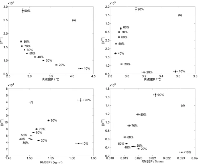
Figure 9. ||bav|| versus RMSEP for (a) T10, (b) T90, (c) specific mass, (d) sulphur. Standard errors are indicated by horizontal and vertical bars.
be able to capture the various vibrational phenomenae involved in the NIR analysis of protein content.
On the other hand, the largest subsampling ratios (80 and 90%) yielded models with considerably high ||bav|| values. In this case, since more calibration samples
were employed, MLR-SPA was able to include a larger number of spectral variables in each individual model, which resulted in an increase in ||bav||. Therefore, although
suitable RMSEP values were obtained, the resulting MLR-SPA-subagging models are more sensitive to noise in the spectral measurements. This feature would compromise prediction accuracy if the models were applied to new measurements with lower signal-to-noise ratio, as illustrated elsewhere.20
In view of the above discussions, by taking into account
the results of ||bav|| and RMSEP for both properties, the
most suitable subsampling ratios would be in the range 40-60%.
Diesel data set
As in the two case studies above, a marked improvement
in RMSEP and ||bav|| was observed for all diesel properties
as the number of iterations was increased up to P = 30. Therefore, the corresponding graphs are omitted for brevity. The average results obtained for different subsampling ratios with P = 30 are shown in Figure 9. Again, the worst
results in terms of either RMSEP or ||bav|| were always
obtained for the extreme values of q (10 and 90%). On the overall, the best results for these two metrics were obtained for q ranging from 30 to 50%.
Conclusions
as well as near-infrared spectrometric determination of moisture and protein in wheat and distillation temperatures (T10 and T90), specific mass and sulphur in diesel were carried out. The results were evaluated in a multi-criterion framework by considering prediction ability (RMSEP)
and sensitivity to spectral measurement noise (||bav||). In
view of these metrics, it was found that 30 subsampling iterations were sufficient to obtain convergence of the MLR-SPA-subagging procedure, which is in agreement
with the findings of a previous study.12 The best results
were obtained for subsampling ratios in the range 20-40% (simulated data), 40-60% (wheat) and 30-50% (diesel). Therefore q = 40% is found to be an appropriate
compromise choice. In terms of the number Ncal of
calibration samples, these q percentages correspond to 20-40 samples (simulated data), 28-42 samples (wheat) and 26-43 samples (diesel). The smaller number of calibration samples required for the simulated dataset can be ascribed to the fewer sources of variability as compared to the wheat and diesel datasets, which involve actual physical/ chemical phenomenae. It is worth noting that the range
of Ncal values indicated above for these real-life datasets
is in agreement with the guidelines of the ASTM E 1655
05 standard,24 which recommends the use of at least 24
calibration samples.
Acknowledgments
The authors thank CAPES (PROCAD Grant 0081/05-1 and doctorate scholarship) and CNPq (MSc scholarship and research fellowships) for financial support.
References
1. Araújo, M. C. U.; Saldanha, T. C. B.; Galvão, R. K. H.; Yoneyama, T.; Chame, H. C.; Visani, V.; Chemom. Intell. Lab. Syst. 2001, 57, 65.
2. Liu, F.; Jiang, Y. H.; He, Y.; Anal. Chim. Acta 2009, 635, 45. 3. Li, L. N.; Li, Q. B.; Zhang, G. J.; J. Infrared Milli. Terahz. Waves
2009, 30, 1191.
4. Pereira, A. F. C.; Pontes, M. J. C.; Neto, F. F. G.; Santos, S. R. B.; Galvão, R. K. H.; Araujo, M. C. U.; Food Res. Int. 2008, 41, 341. 5. Nezio, M. S. D.; Pistonesi, M. F.; Fragoso, W. D.; Pontes,
M. J. C.; Goicoechea, H. C.; Araujo, M. C. U.; Band, B. S. F.; Microchem. J. 2007, 85, 194.
6. Breitkreitz, M. C.; Raimundo Jr, I. M.; Rohwedder, J. J. R.; Pasquini, C.; Dantas Filho, H. A.; José, G. E.; Araújo, M. C. U.; Analyst 2003, 128, 1204.
7. Galvão, R. K. H.; Araújo, M. C. U.; Fragoso, W. D.; Silva, E. C.; José, G. E.; Soares, S. F. C.; Paiva, H. M.; Chemom. Intell. Lab. Syst. 2008, 92, 83.
8. Kompany-Zareh, M.; Akhlaghi, Y.; J. Chemom. 2007, 21, 239. 9. Soares, S. F. C.; Galvão, R. K. H.; Araújo, M. C. U.; Silva, E. C.;
Pereira, C. F.; Andrade, S. I. E.; Leite, F. C.; Anal. Chim. Acta 2011, 689, 22.
10. Soares, A. S.; Galvão, R. K. H.; Araújo, M. C. U.; Soares, S. F. C.; Pinto, L. A.; J. Braz. Chem. Soc. 2010, 21, 1626.
11. Soares, A. S.; Galvão Filho, A. R.; Galvão, R. K. H.; Araújo, M. C. U.; J. Braz. Chem. Soc. 2010, 21, 760.
12. Galvão, R. K. H.; Araújo, M. C. U.; Martins, M. N.; José, G. E.; Pontes, M. J. C.; Silva, E. C.; Saldanha, T. C. B.; Chemom. Intell. Lab. Syst. 2006, 81, 60.
13. Bühlmann, P.; Yu, B.; Ann. Statist. 2002, 30, 927.
14. Martins, M. N.; Galvão, R. K. H.; Pimentel, M. F.; J. Braz. Chem. Soc. 2010, 21, 127.
15. Kalivas, J. H.; Chemom. Intell. Lab. Syst. 1997, 37, 255. 16. Forina, M.; Lanteri, S.; Casale, M.; Oliveiros, M. C. C.;
Chemom. Intell. Lab. Syst. 2007, 87, 252.
17. Beebe, K. R.; Pell, R. J.; Seasholtz, B.; Chemomics - A Pratical Guide, Wiley: New York, 1998.
18. Honorato, F. A.; Galvão, R. K. H.; Pimentel, M. F.; Neto, B. B.; Araújo, M. C. U.; Carvalho, F. R.; Chemom. Intell. Lab. Syst. 2005, 76, 65.
19. Kennard, R. W.; Stone, L. A.; Technometrics 1969, 11, 137. 20. Pinto, L. A.; Galvão, R. K. H.; Araújo, M. C. U.; Anal. Chim.
Acta 2010, 682, 37.
21. Kalivas, J. H.; Anal. Chim. Acta 2004, 505, 9.
22. Stout, F.; Baines, M. R.; Kalivas, J. H.; J. Chemom. 2006, 20, 464.
23. Papoulis, A.; Probability, Random Variables, and Stochastic Processes, McGraw-Hill Kogakusha: Tokyo, 1965.
24. Annual Book of ASTM Standards; Standards Practices for Infrared, Multivariate, Quantitative Analysis, ASTM International E1655, West Conshohocken: Pennsylvania, USA, 2000, vol. 03.06.
Submitted: March 23, 2011
Published online: September 15, 2011