Abstract—In this work, we analyze modified bowtie nanoantennas
with polynomial sides in the excitation and emission regimes. In the excitation regime, the antennas are illuminated by an incident plane wave, and in the emission regime, the excitation is fulfilled by infinitesimal electric dipole positioned in the gap of the nanoantennas. Several antennas with different sizes and polynomial order were numerically analyzed by method of moments. The results show that these novel antennas possess a controllable resonance by the polynomial order and good characteristics of near field enhancement and confinement for applications in enhancement of spontaneous emission of a single molecule.
Index Terms— Nanoantennas; modified bowtie nanodipoles; near field enhancement; spontaneous emission; method of moments.
I. INTRODUCTION
Nanoantennas are metal nanostructures used to enhance, confine, receive, and transmit optical
fields [1]. Potential applications of nanoantennas are ultra-high-density optical data storage devices
[2], super-resolution microscopy [3], integrated nano-optical devices [4], optical communication
between functional elements of nanometer size [5], chemical enhancement for surface-enhanced
Raman scattering [6], and biology [7]. Increasing investigations in this field in the last years is due to
the promising applications, the development of modern techniques of micro and nanofabrication tools
such as focused ion beam milling (FIB), and increasing the capabilities of numerical techniques of
analysis.
One important application of nanoantennas is to enhance the spontaneous emission of a single
molecule. In this process, a molecule positioned near a given antenna is excited by the high local field
of the antenna. The analysis of this process can be divided in two regimes: excitation and emission
ones. In the first regime, an incident plane wave illuminates the antenna and the near field
enhancement is the phenomenon to be investigated. In the second regime, the emitter localized near
the antenna is modeled by an infinitesimal electric dipole, and the radiation efficiency is the object of
interest. The whole emission performance of the emitter depends on these two processes. Analysis of
linear and bowtie nanoantennas for the enhancement of spontaneous emission are given in [8], [9].
In this paper, we present an analysis of Au modified bowtie nanoantennas in the excitation and
emission regimes. The proposed antennas possess polynomial sides instead of linear of the
conventional triangular antenna. We numerically study several modified antennas with different sizes
Analysis of Modified Bowtie Nanoantennas in
the Excitation and Emission Regimes
Karlo Q. da Costa, Victor A. Dmitriev,
and polynomial order by method of moments (MoM). The analyzed parameters are: spectral response,
resonances, near field enhancement and confinement, radiation efficiency and directivity.
II. THEORY
A. Geometries of the Modified Bowtie Nanantennas
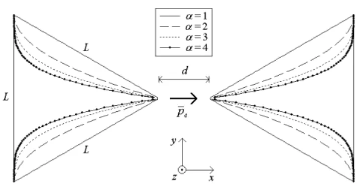
The geometries of the modified bowtie nanoantennas are shown in Fig. 1. In this figure, four
antennas made of Au with different values of the parameter α=(1,2,3,4) are presented, where α is the
polynomial order of the sides variation. The polynomial function used to model the curvature of the
sides is x=(y/k1)α, where k1=L/2h 1/α,
h=0.5L(3)0.5, L is the side length of the conventional bowtie
triangle. The conventional bowtie antenna corresponds to the case α=1 where the side variation is
linear. These antennas are placed in the origin of the coordinate system with the axis of the antenna
oriented along the x axis. The distance between the arms of the bowtie dipoles is d, and the thickness,
which is not shown, is w. With these parameters, the total antenna’s length is d+2×h. For higher
values of α, the tips of the antenna are more acute.
Fig. 1. Geometries of the bowtie nanoantennas with polynomial sides. The form of the sides varies as the function x=(y/k1)α,
where k1=L/2h1/α, h=0.5L(3)0.5. The conventional bowtie antenna corresponds to α=1.
B. Numerical Model of Analysis
The nanoantennas shown in Fig. 1 were numerically analyzed by a MoM code based on model
proposed in [10]. In this model, the equivalent polarization current inside the total volume v of the
antennas
[
(r) 0]
E(r) (r)E(r)j
Jeq= ωε −ε =τ (1)
is determined by solving the tensor integral equation for the electric field
) ( ) , ( ) ( ) ( ) ( 3 ) (
1 , , ,
0 r E dv r r G r E r PV r E j r i
v ⋅ =
−
+
∫
τωε
τ
(2)
In (2), PV means the principal value of the integral where the evaluation is inside the volume v
in (1)-(2) are as follows: i
E and E are the incident and total electric field inside the volume v,
respectively, ω the angular frequency, k0=ω(µ0ε0)1/2=2πc/λ the wave number, λ is the wavelength, c is
the speed of the light in free space, µ0 the free space permeability, ε0 the free space permittivity. The
complex permittivity of the Au particles is ε=ε0εr, where εr is defined
∞ + + − + Γ − − = ε γω ω ω ω ω ω ω ε j j p p
r 2 2
0 2 2 2 2 1
1 (3)
and the parameters of this equation are: ε∞=6, ωp1=13.8×10¹⁵s
−1
, Γ=1.075×10¹⁴s−1, ω0=2πc/λ0,
λ0=450nm, ωp2=45×1014s−1, and γ=9×10¹⁴s−1 [1]. This model is a good approximation in the range of
wavelengths from 500 nm to 1000 nm. Exactly in this frequency range we fulfill our analysis.
The excitation of the antennas is represented by i
E . Two kinds of sources are considered in this
model: an Ex-polarized, z-directed plane wave, and an infinitesimal electric dipole with moment
positioned in middle of the gap’s antenna and polarized in the x axis (Fig. 1). The first numerical
experiment is called the excitation regime and the second the emission regime.
To solve these scattering problems by MoM, the volume of a given antenna is divided in N small
cubic subvolumes, where the total electric field is approximately constant. With this approximation,
the integral equation is transformed into a linear system with Nt=3N equations because there are three
electric field components in each subvolume.
C. Definitions of the Parameters Analyzed
The solution of the equivalent linear system produces the total electric field E inside the volume v
of the antenna. With this result, the near and far field characteristic parameters of the antennas are
calculated. In the excitation regime, we calculated the near electric field and scattering cross section
respectively by
∫
⋅ + = v it r E r r E r G r r dv
E ( ) ( ) τ( ') ( ') ( , ') ' (4)
2 | | ) , ( 8 ) , ( i E U
SCS θ φ = πη θ φ (5)
where η is the free space impedance and U(θ,φ) is the radiation intensity of the scattered far field in a
given direction θ and φ. Other characteristics analyzed in this regime are the field enhancement and
spatial confinement. The first one is defined by (|E|/|E0|)
2
, where |E| is the total field near the antenna
and |E0| is the amplitude of the incident plane wave. The second characteristic is a spatial distance
between 3dB points where (|E|/|E0|)
2
=0.5. This parameter is a spatial bandwidth (in nanometers)
around the maximum field enhancement, where in the case of the nanoantennas, this maximum value
is in the middle of the antenna’s gap. In the present analysis, we calculated the spatial confinement in
In the emission regime, we evaluated the directivity and radiation efficiency respectively by [11]
rad P U
D(θ,φ)=4π (θ,φ)/ (6)
) /(
100
(%) Prad Ploss Prad
e = × + (7)
where Prad and Ploss are the radiated and dissipated power of the antennas. In (6) the characteristic U is
the total radiation intensity due to the scattered field by the antenna and the radiated field by the
infinitesimal electric dipole.
III. NUMERICAL RESULTS
Based on theory presented in the previous section, several codes in Fortran and Matlab were
developed. The modified nanoantennas with α=(1,2,3,4) were simulated with Nt=4608, 5460, 6516,
and 7896, respectively. With these discretizations we have a good convergence of the results. The
dimensions used in these simulations are L=50nm, d=10nm, and thickness w=9.5; 10; 10.3; 10.6 (nm)
for the antennas with α=(1,2,3,4) respectively. We also simulated nanoantennas with α=3 for different
values of L and d. In these simulations, eight nanoantennas were analyzed with L=75; 100; 125; 150
(nm) for fixed d=10nm, and d=5; 15; 20; 25 (nm) for fixed L=50nm. The following sections present
the results.
A. Spectral Response in the Excitation Regime
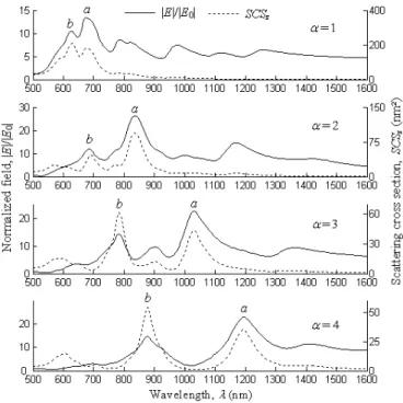
Fig. 2 shows the spectral response of the normalized field (|E|/|E0|) in the middle of the antenna’s
gap (the origin of the coordinate system) and the scattering cross section in the +z direction (SCSz) of
the modified bowtie nanoantenna with α=(1,2,3,4). These characteristics were obtained by (4) and (5)
in the excitation regime. We observe in these results two principal resonances in λa and λb (λa>λb),
which are the same for the near field (|E|/|E0|) and far field (SCSz).
These resonances are shifted to the right for large values of α, but the variation of λa is higher than
λb. We conclude that the resonance λa is more sensitive with the geometric parameter α than the
resonance λb, and this parameter can be used to tune the resonance of a particular antenna.
The values of |E|/|E0| and SCSz at the resonances λa and λb are different. In the near field region, the
main resonance is λa, where it presents highest values of |E|/|E0|. In the far field region, the maximum
values of SCSz are obtained in λb, the exception is the case α=2 (Fig. 2). Table I summarizes the
values of some parameters of these antennas at the resonance λa. This table shows that the modified
dipoles with α=(2,3,4) have higher field enhancement than the conventional one (α=1), and the
highest value is 692 of the case α=2. The scattering cross section of antennas with larger values of α
are smaller, this is due the different physical areas of the antennas. The spatial confinement presented
Fig. 2. Spectral response of the normalized field in the middle of the antenna’s gap and scattering cross section in the direction +z of the modified bowtie nanoantennas with α=(1,2,3,4) with L=50nm and d=10nm.
TABLE I. PARAMETERS OF THE MODIFIED BOWTIE NANODIPOLES
Parametera Modified Bowtie Nanoantenna
α α α
α=1 αα=2 αα αααα=3 αααα=4
Resonant wavelength, λa (nm) 675 840 1030 1194
Field enhancement, (|E|/|E0|)2 180 692 508 524
Scattering cross section, SCSz (nm²) 180 93 44 35
Spatial confinement in y, σy (nm) 7.7 5.8 6.9 7.6
Spatial confinement in z, σz (nm) 11 10.4 11 11.8
a. These parameters were calculated at resonance λa.
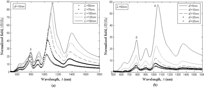
Fig. 3 presents the dependence of the spectral response of the antenna with α=3 on the lengths L
and d. The parameter shown in these figures is the normalized field |E|/|E0| in the middle of the
antenna’s gap. Fig. 4 shows the variation of the normalized field and resonant wavelength λa versus
the total antenna’s length 2×h+d and the distance between the arms of the dipole d. We observe in
these figures that when the size of the antenna is increased, the main resonance λa and the normalized
field are linearly increased. On the other hand, the variation of these parameters with d are nearly
constant for λa, and approximately exponential for |E|/|E0|, where for lower distances d, this
normalized field increases rapidly.
B. Near Field Distributions
In this section, we analyze the electric field distributions near the nanoantennas and its spatial
confinement properties. Fig. 6 shows the variation of the normalized total field near the nanoantennas
because the antenna’s thickness are variable, i.e. w=9.5; 10; 10.3; 10.6 (nm) for the antennas with
α=(1,2,3,4) respectively. The dimensions of the antenna are L=50nm and d=10nm, and the
wavelength where these distributions were calculated are the resonances λa given in Table I. In this
figure, we observe the better field confinement of the modified antennas than that for the conventional
one.
Fig. 3. Variation of the spectral response of the normalized field in the middle of the antenna’s gap for the nanoantenna with
α=3. (a) variation with the length L. (b) variation with the length d.
Fig. 4. Variation of the normalized field and resonant wavelength λa versus the total antenna’s length 2×h+d (upper) and distance between the arms of the nanoantenna d (down). These results are for the antenna with α=3.
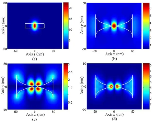
The fields shown in Fig. 5 are the total field, but we also analyzed the distributions of the isolated
components x, y, and z for the antenna with α=3. The results are presented in Fig. 6, where we
observe that the values of the components x and z are larger than the component y in the plane
z=10nm (Fig. 6(b)-(d)), and the x component (Fig. 6(b)) is more confined in the antenna’s gap. We
6(a)). From these results, we conclude that in the antenna’s gap, the principal polarization is the
component x. If a molecule is positioned in the middle of this dipole, the antenna’s field will excite in
the molecule a electric dipole moment px, this is why we analyze in this paper only this polarization.
The results of this emission regime will be presented in the next section.
Fig. 5. Normalized near field |E|/|E0| distribution at the plane z=10nm of the modified nanoantennas with (a) α=1, (b) α=2,
(c) α=3, and (d) α=4, L=50nm and d=10nm.
Fig. 6. Near field distributions of the nanoantenna with α=3. (a) |Ex|/|E0| in yz, and (b) |Ex|/|E0|, (c) |Ey|/|E0|, (d) |Ez|/|E0| in
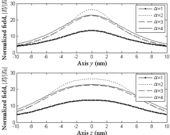
To analyze the spatial confinement of the results presented in Fig. 5 and Fig. 5(a), we present in
Fig. 7 the variation of the normalized field along the axis y and z. The results of the spatial
confinement parameters σy and σz are presented in Table I. We note that these antennas possess higher
confinement along the axis y than the axis z, and the highest confinement in the axis y is for the
modified antennas with α=2, where σy=5.8nm. The confinement in the axis y depends on the value of
the polynomial order (α), and the confinement in the axis z depends on the antenna’s thickness (w).
All the antennas in Fig. 6 possess approximately the same values of w, this is why they have similar
values of σz.
Fig. 7. Near field distributions |E|/|E0| of the nanoantennas with α=(1,2,3,4) along the axis y (upper) and z (down).
C. Directivity and Efficiency in the Emission Regime
In this section, we present the numerical results of the modified bowtie nanoantennas in the
emission regime, where an infinitesimal electric dipole localized in the middle of the nanoantennas is
the source of the antenna system (Fig. 1). The polarization of this infinitesimal dipole is in the x
direction and its moment dipole is px. This polarization was chosen because in the excitation mode
only the component x of the electric field exists in the middle of the bowtie nanoantennas (Fig. 6).
The results presented here are the directivity (D) in the +z direction (θ=0o) and the radiation efficiency
(e) as defined in (6) and (7) respectively.
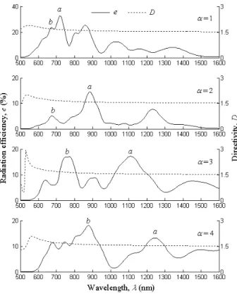
Fig. 8 presents the spectral response of D and e of the bowtie nanoantennas with α=(1,2,3,4), for
L=150nm and d=10nm. The results of e show that the maximum efficiency of each antenna occurs at
the same resonant wavelengths λa and λb of the excitation regime. We also observe that the
efficiencies in these resonances are reduced for larger values of α, i.e. antennas with same dimensions
L and d but higher near field enhancements have smaller radiation efficiency. These results are in
accordance to those previously observed for conventional bowtie nanoantennas with different radius
Fig. 8. Radiation efficiency and directivity in +z direction versus wavelength of the nanoantennas with α=(1,2,3,4), for L=150nm and d=10nm.
With respect the results of D in Fig. 8, all the antennas possess D≈1.5 at the resonances λa and λb,
this shows that these antennas have a radiation diagrams similar to that of an infinitesimal dipole in
these resonances. The values of D near the wavelength λ=550nm are a little different of 1.5. We
believe this is due the plasma resonance of Au, but this effect is not important in the analysis because
it occurs far from the resonance of the antennas, where the radiation efficiency is very small. In
resume, the radiation characteristics of these antennas are similar to those of electrically small
antennas, because the total length 2×h+d of them are smaller than the resonant wavelengths λa and λb,
so their directivities are constant in a wide range of wavelengths analyzed.
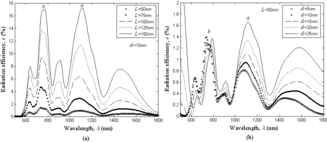
To investigate the dependence of e on the dimensions L and d, Fig. 9 show the variation of the
spectral response of the radiation efficiency in function of the sizes L and d. These results were
obtained for the nanoantenna with α=3, d=10nm in Fig. 9(a) and L=50nm in Fig. 9(b). We observe
that the maximum efficiency also occur in the same resonant wavelengths (λa and λb) of the excitation
regime presented in Fig. 4. For larger values of L with d fixed, we have better radiation efficiency,
and for larger d with L fixed, we also have higher efficiency.
Fig. 10 presents the variation of e at the resonances λa and λb in function of the total length 2×h+d
and d. The results of these figures shows that the radiation efficiency is very small for nanoantennas
with L=50nm, for example in d=10nm the efficiency is e<1%, but it increases exponentially with d.
This approximate exponential variation is for the resonance λa, and for the resonance λb the efficiency
Fig. 9. Variation of the spectral response of the radiation efficiency of the nanoantenna with α=3. (a) with the length L for d=10nm. (b) with the distance d for L=50nm.
Fig. 10. Variation of the spectral response of the normalized field in the middle of the antenna’s gap for the nanoantenna with α=3. (a) variation with the length L. (b) variation with the length d.
The increasing of e with 2×h+d is approximately linear for the two resonances λa and λb, where if,
for example, the total length is increased by a factor of two, the efficiency is also increased two times.
With the results presented in this section, we conclude that the modified bowtie nanoantennas with
α>1 possess smaller radiation efficiency than that of the conventional one with α=1 and their
directivities are equal to 1.5 at the principal resonances. However, we can rise up the radiation
efficiency with the increasing of the dimensions L and d.
IV. CONCLUSIONS
In this paper, we presented a theoretical analysis of modified bowtie nanoantennas with polynomial
sides in the excitation and emission regimes. We observed in the excitation regime that the resonances
gap’s antenna is increased, where it presents only polarization along the axis of the dipoles. Also, the
field confinements of the modified antennas are higher than the conventional one. In the emission
mode, we noted that the maximum radiation efficiency of all antennas occurs at the same resonant
wavelengths obtained in the excitation regime, and the values of these efficiencies, for the modified
antennas, are smaller than those of the conventional one with same dimensions, but it can be increased
for larger antenna’s size and gap distances between the arms of the dipoles. With respect the directive
properties of these antennas, all the cases analyzed presented directivities similar to that of an
electrically small antenna.
With all these results, we conclude that the modified bowtie nanoantennas have higher near field
enhancement and confinement, and smaller radiation efficiency than those of the conventional bowtie
antenna with linear sides. With appropriated dimensions, these novel nanoantennas can be used, for
example, to enhance the spontaneous emission of single molecules positioned in the middle of the
antenna’s gap. Future works can be the analysis the characteristics dependence of these antennas on
the thickness, orientation of the incident plane wave, and the polarization of the emitter in the gap.
ACKNOWLEDGMENT
This work was financially supported by the Brazilian agency National Counsel of Development
Scientific and Technologic - CNPq by contract number 151731/2008-0.
REFERENCES
[1] L. Novotny, and B. Hecht, Principles of Nano-Optics, New York: Cambridge, 2006.
[2] H. Wang, C. T. Chong, and L. Shi, “Optical antennas and their potential applications to 10 terabit/in² recording,” Optical Data Storage Topical Meeting, pp. 16-18, May 2009.
[3] O. Sqalli, I. Utke, P. Hoffmann, and F. M.-Weible, “Gold elliptical nanoantennas as probes for near field optical microscopy,” J. of Appl. Physics, vol. 92, pp. 1078-1083, July 2002.
[4] S. E. Lyshevski, and M. A. Lyshevski, “Nano- and microopto-electromechanical systems and nanoscale active optics,” Third IEEE Conference on Nanotechnology, August 2003.
[5] J.-S. Huang, T. Feichtner, P. Biagioni, and B. Hecht, “Impedance matching and emission properties of nanoantennas in an optical nanocircuit,” Nano Lett., vol. 9, pp. 1897-1902, April 2009.
[6] D. P. Fromm, A. Sundaramurthy, A. Kinkhabwala, P. J. Schck, G. S. Kino, and W. E. Moerner, “Exploring the chemical enhancement for surface-enhanced Raman scattering with Au bowtie nanoantennas,” The J. of Chemical Phisics, vol. 124, 2006.
[7] M. F.G.-Parajo, “Optical antennas focus in on biology,” Nat. Photonics, vol. 2, pp. 201-203, April 2008. [8] J.-W. Liaw, “The quantum yield of a metallic nanoantenna,” Appl. Phys. A, vol. 89, pp. 357-362, 2007.
[9] J.-W. Liaw, “Analysis of a bowtie nanoantenna for the enhancement of spontaneous emission,” IEEE J. Selected Top. Quantum Electronics, vol. 14, pp. 1441-1447, December 2008.
[10]D. E. Livesay, and K. M. Chen, “Electromagnetic fields induced inside arbitrary shaped biological bodies,” IEEE Trans. Micro. Theo. Thec., vol. 22, pp. 1273-1280, December 1974.