ABSTRACT: Autonomous star trackers are optical-electronic devices used for attitude determination of artiicial satellites, having as a reference for this computation the positions of stars. There is one autonomous star tracker in development at the Aerospace Electronics Division of the Brazilian National Institute for Space Research. The autonomous star tracker imager is a complementary metal-oxide-semiconductor active pixel sensor, consisting of an integrated circuit with an array of them. Each pixel has a photodetector and an active ampliier. Since it has many ampliiers, the active pixel sensor has an additional ixed pattern noise, therefore its characterization is different from the traditional method used for the charge coupled devices. With this experiment, it was observed that the mean value per columns of ixed pattern noise is ~100% greater than the mean value of the pixel one. Taking into account this result, modeling the pixel ixed pattern noise will not be important to improve the autonomous star tracker sensibility. Furthermore, the random noise value was less than 1% of the ixed pattern noise range data, being possible to estimate it. In this work, we presented the ixed pattern noise new parametric model, which has a good agreement when compared with the experimental data. It was calculated Pearson’s product-moment correlation coeficient between the model and the observed data, in order to quantify the model accuracy and it was obtained 99% for lat ield and 79% for dark current.
KEYWORDS: Star trackers, Aerospace systems, Attitude determination, Spacecraft, Applied astronomy.
Determining the Fixed Pattern Noise of a
CMOS Sensor: Improving the Sensibility of
Autonomous Star Trackers
Eduardo dos Santos Pereira1
INTRODUCTION
Autonomous star trackers (AST) are optoelectronic instruments used for attitude determination of a satellite by observing stars (Liebe, 1995, Liu et al., 2011). he precision of attitude determination depends on the accuracy of the AST image registration. hus, the calibration of a ixed pattern noise (FPN) of the AST image sensor has an important role. he FPN is a variation in the output pixel values, under uniform illumination, due to device and interconnection mismatches across an image sensor. In the case of complementary metal-oxide-semiconductor (CMOS) sensors, passive and active pixel (PPS and APS), there are several ampliiers in which some are shared by pixels and others are not. hereby, in order to determine the FPN, it is necessary to take into account not only the pixel noise, but also that of the column (Gamal et al., 1998, Bigas et al., 2006). On the other hand, Schöberl et al. (2009) showed that it is possible to model the FPN as a function of the image acquisition integration time, with a nonlinear parametric model. However, for that model, it is necessary to ind a set of parameters for each pixel, and for a 6 MPixel sensor 75 Mbytes are required to save those data. Another issue presented by Schöberl et al. (2009) is concerning the fact of assuming dark current as a constant for each pixel as the model of Pillman et al. (2006) for describing the FPN with a linear algorithm. However, these authors also presumed that the segmented linear and quadratic models have a better characterization of the FPN than a pure linear one.
In this work, we were mainly interested in determining and modeling the FPN of the CMOS used in the AST. his
1.Instituto Nacional de Pesquisas Espaciais – São José dos Campos/SP – Brazil
Author for correspondence: Eduardo dos Santos Pereira | Instituto Nacional de Pesquisas Espaciais, Divisão de Eletrônica Aeroespacial | Avenida dos Astronautas, 1.758 – Jardim da Granja | CEP 12.227-010 – São José dos Campos/SP – Brazil | E-mail: [email protected]
procedure would allow us to perform a data correction before starting the process of pattern recognition from stars. Such review will improve the sensibility of the AST and therefore reduce errors on the satellite attitude determination.
AUTONOMOUS S TAR SENSOR
h e AST consists of a pinhole imaging system that measures the direction vector of a star in its own reference frame (Zenick, 2003, Xing et al., 2006, Liu et al., 2011). Firstly, the stars into the i eld of view (FOV) are registered by the CMOS APS, secondly they are recognized by a pattern recognition routine. Finally, the stars are compared with an internal catalog and the attitude matrix of the AST is calculated. In Fig. 1 a simplii ed block diagram of AST functionality is presented.
For the calculus of AST attitude matrix, M, it is necessary to know a vector direction, v, of the star in an inertial frame. h e value of v is obtained from the right ascension, α, and
declination, δ, from a master catalog, as Eq. 1:
v = vx vy vz
cos(α) cos(δ) sin(α) cos(δ)
sin(δ)
⎡ ⎣ | ⎡
⎣ | ⎡
⎣
| ⎡
⎣ |
= . (1)
h en, a new catalog is generated. h e attitude matrix should satisfy (Eq. 2):
W = Mv , (2)
where W is the vector direction of stars into the AST reference frame, which is given by Eq. 3 (Xing et al., 2006 and Liu et al., 2011):
W = 1
-(x-x0) -(y-y0)
f
⎡
⎣ ⎡
⎣
√(x-x0)2(y-y
0)
2+f2 , (3)
where x0 and y0 represent the intersection points of the focal plane and the optical axis; x and y are the observed star locations on the detector plane and ƒ is the focal length of the AST camera. In Fig. 2 an illustration of the AST reference, o, and inertial frames, O’, is presented.
Usually, the matrix M can be estimated by minimizing the least-square error (Eq. 4):
L = 1
2 ∑ ai||Mvi - Wi||
2
i= 1 n
,
(4)
where a’i are the weights and n is the number of observations. h is equation is also called Wahba’s problem (Wahba, 1965).
Pinhole Lens
Image
Processor Pattern
Recognition Software Active
Pixel CMOS Imager Field of
View
Star Catalog
Attitude Estimation
(x, y, z)
Figure 1. Simplii ed block diagram of a star tracker. Adapted from Zenick (2003).
Zn
Xn
Yn Lens system
Wi
Wj
θij
Z
x
(x0, y0) o
y ƒ
O’
Figure 2. Star tracker measurement. The O represents the inertial referential frame and O’ is the autonomous star trackersreferential frame. Adapted from Liu et al. (2011).
E STIMATION AND MODELING
THE FIXED PATTERN NOISE
Yj = 1 N i=∑ 1Fij
N
, (5)
Xij =Fij - Yj , (6)
where Fij is an average estimator that is obtained from a sample of AST images, and N is the number of columns of the images. Fij is determined as follows:
• obtain a sample of k images from the AST;
• in order to reduce the random noise, the mean value of the sample should be calculated;
• from the result of the image, the average value of all pixels is found;
• Fij is determined through the subtraction from the mean image of the average value of all their pixels, each at a time.
he variances, by column and pixel, are presented in Eqs. 7 and 8:
σ2 = 1
M- 1j=∑ 1Yj
M 2
Y , (7)
σ = 1
M(N - 1) j=∑ 1Xij
M 2
2
x ∑
i=1
N
. (8)
Furthermore, we consider the normalized root mean square error (NRMSE) for each image of the sample in order to determine the predominance of the random error. herefore, this allows us to know if it is possible to make a FPN correction. In the present case, a residual value of each image, Rijk
, was obtained by subtracting the average value of all the pixels, each at a time, from the image k. he NRMSE of FPN by columns and pixels is in Eqs. 9 and 10:
Ck = 1
max(Yj) -min(Yj)
Rijk
rms ∑
j=1 N
1
N
1
N - Yj
2 ∑
i=1 N
(9)
Pk = 1
max(Xj) -min(Xj) Rij k
rms ∑
i=1 M 1
MN
1
N
-2
∑ i=1
N ∑
j=1 N
Rijk- X
ij . (10)
In this work, we modeled the FPN columns tendency as a third-order polynomial function (Eq. 11),
fc(x) = a0 + a1x + a2x2 + a 3x
3 , (11)
and based on the work of Schöberl et al. (2009), we considered a it of the FPN columns as a function also of the integration time as Eq. 12:
Ffpn(x,τ) = fc(x)gc(τ) , (12)
where τ represents the integration time, and gc(τ)=b0+b1τ+b2τ2 and ai, bi are parameters to be determined. However, in the work of Schöberl et al. (2009), the set of parameters found were for each individual pixel. Herein, we are more interested in modeling the column FPN using only one function for all columns and integration time range.
In order to determine ai, bi, we minimize the least-square error as in Eq. 13:
J(a, b) =1
2∑l
2 ||Yjl - Ffpn(a, b, xj, τl)|| ∑
j , (13)
where a=[a0, a1, a2, a3], b=[b0, b1,b2], and Yjl are the FPN
columns given by Eq. 13 for l diferent integration times. In order to quantify the model it accuracy, using Eq. 12 and setting the best it parameters to compare with the experimental data, we have considered Pearson’s product-moment correlation coeicient (Press et al., 1993), as seen in Eq. 14:
ρ =
∑
l(Yjl - Y)
2
∑
j
∑
l (Yjl - Y)
∑
j
∑
l (Ffpn, jl - Ffpn) 2
∑
j
(Ffpn, jl - Ffpn)
, (14)
being Y the mean value of Yjl , Ffpn, jlis given by Eq. 12 for x j, τl and Ffpn is the mean value of Ffpn, jl.
RESULTS
AST sensibility. Taking into account these results, in this work we focused our attention on the column FPN modeling.
Figure 3 shows the total FPN estimated, Fij, in (A) and the pixel one, in (B). It is noteworthy that the value of the pixel FPN is the Fij subtracted from the column FPN. h ese results are for 200 msec of integration time. It is also possible to observe vertical lines in the image in A, which are the FPN column, and their values are plotted in Fig. 4. h e highlighted line in Fig. 3 is a defective column in our APS. h is column is not considered for the FPN analyses.
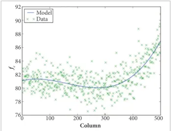
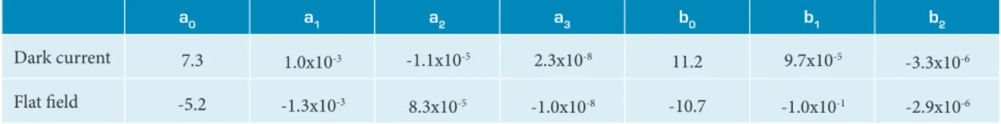
Figures 4 and 5 show the FPN per columns for dark current (l at i eld), the continuous line is the polynomial modeling of the column FPN, given by Eq. 11. In these cases, the vector of parameters that provide us a better i t is presented in Table 1.
In Figs. 6 and 7 the normalized root mean square error of FPN per column estimated for each image of the sample for dark current and l at i eld is represented. In both cases, the integration time was 200 msec. h ese i gures represent the general behavior of the random noise from image to image, when compared to the FPN range amplitude. In general, the random noise, or error of FPN, has a value lower than 1% with respect to FPN range amplitude.
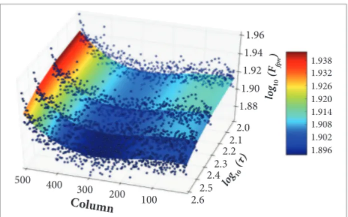
h e Figs. 8 and 9 demonstrate the last-square i t of the Eq. 12 for dark current and l at i eld, respectively. h e set of best i t parameters are given in Table 2.
Pearson’s product-moment correlation coei cients, given by Eq. 14, were obtained for dark current (0.7947) and l at i eld (0.9995).
h ese results show that we had a good agreement with the modeling i t when compared with the experimental data. h is means that we have 99.95% of accuracy in modeli ng the l at i eld column FPN and 79,47% of accuracy in the dark current model for the column FPN.
Table 1. Best i t parameters set for modeling i xed pattern
noise columns.
a0 a1 a2 a3
Dark current 8 1 .9 8 .5 x1 0-3 -1. 1x 10⁻⁴ 2.0x10⁻⁷
Flat i eld 1 6 8 .0 5.5x10⁻² -3.5x10⁻⁴ 4.3x10⁻⁷
The column i xed pattern noise (FPN) has different behaviors when the dark current FPN is compared to the l at i eld one. As the FPN is distinct for each sensor, we expect different sets of parameters for varied complementary metal-oxide-semiconductor sensors.
For this work, a sot ware tool, called FPNAnalyser© was developed for analyzing and modeling the FPN. h is program was based on all the theories about FPN determination presented here. h e i rst tab of the Graphical Using Interface of FPNAnalyser© is shown in Fig. 10. It will be released as an
Figure 4. Column i xed pattern noisefor dark current and 200 msec of integration time.
92
90
88
86
84
82
fc
Column
0 100 200 300
80
78
76
Model Data
400 500
The continuous line is the polynomial modeling.
Figure 3. High brightness and contrast image of dark current for 200 msec of integration time. Total i xed pattern noise estimation (A) and pixel i xed pattern noise(B).
A B
The bright column to the right is the defective of the APS, which is not being taking into account for the i xed pattern noisemodeling.
Figure 5. Column i xed pattern noisefor l at i eld and 200 msec of integration time.
174
172
170
168
166
164
fc
Column
0 100 200 300
162
160
158 Model
Data
4 0 0 5 0 0
156
Figure 6. Normalized root mean square error for dark current and 200 msec of integration time.
0.07
0.06
0.05
0.04
0.03
k Image
0 5 10 15
0.02
0.01
0.00
20 25 30 35 40
C
k τm
s
Figure 7. Normalized root mean square error for l at i eld and 200 msec of integration time.
0.07 0.08 0.09
0.06
0.05 0.04
0.03
k Image
0 5 10 15
0.02
0.01
0.00
20 25 30 35
C
k τm
s
Figure 8. Least-square i t of the i xed pattern noisecolumn considering dark current.
1.938
1.96
1.932 1.926 1.920
lo
g (10 Ffpn
)
C o l u mn200 100 300
1.914 1.908 1.902
400 500
1.896
1.94
1.92
1.90
1.88
2.0 2.1 2.2 2.3 2.4 2.5 2.6
l og 1 0
(τ)
The integrating time, τ, is in msec. This surface was obtained using Eq. 13. The scattered points are experimental data.
Figure 9. Least-square i t of the i xed pattern noisecolumn considering l at i eld.
2.40
2.4
2.36 2.32 2.28
lo
g10
(F
fp
n
)
Column
100 200 300
2.24 2.20 2.16
400 500
2.12
2.3
2.2
2.1
2.02.1 2.22.3
2.42.5 2.6
log10 (τ)
The integrating time, τ, is in msec. This surface was obtained using Eq. 13. The scattered points are experimental data.
Table 2. Set of best it parameters for ixed pattern noisecolumns models as a functional of integration time.
a0 a1 a2 a3 b0 b1 b2
D a r k c u r r e n t 7.3 1 .0 x 1 0 - 3 -1.1x10⁻⁵ 2.3x10⁻⁸ 11.2 9.7x10⁻⁵
-3.3x10⁻⁶
F lat ield -5.2 -1.3x10⁻³ 8.3x10⁻⁵ -1.0x10⁻⁸ -10.7 -1.0x10⁻¹ -2.9x10⁻⁶
open source under the general GNU license version 3 (see http://www.gnu.org/licenses/gpl-3.0.txt for more details).
DISCUSSION AND CONCLUSION
It was presented a general concept of AST and a way to evaluate the FPN of CMOS APS used as the AST image. he determination of the FPN is important to achieve not only higher precision of observations of greater magnitude stars (less bright stars), but also to perform corrections of the brightness of low magnitude stars. he attitude determination depends on the precision of stellar identiication, therefore the FPN correction leads to a better knowledge of this attitude.
With this experiment, it was observed that the mean value per FPN columns is greater than that of the pixel FPN. Thus, it is relevant only the FPN column for doing the APS image correction. Also, we showed that the parametric model of FPN columns, as function of columns and integration time, had a good agreement with experimental data. This fact was quantified by Pearson’s
product-moment correlation coefficient. We obtained 99.95% of accuracy for flat field and a 79.47% for dark current. We strongly suggest future works including the development and implementation of the correction algorithm of FPN columns for the AST.
he greatest contribution of this work is the applied methodology, since it was widely detailed in a single paper, i.e., a FPN correction analysis for an AST image. Another point is that we have developed a sotware tool that could be used not only for modeling the FPN, but also to trace strategies for doing an automatic image correction by an embedded system into the AST image.
ACKNOWLEDGEMENTS
Eduardo S. Pereira would like to thank the C o nselho Nacional de Desenvolvimento Cientíico e Tecnológico (CNPQ) for their inancial support (process: 382477/2012), Instituto Nacional de Pesquisas Espaciais (INPE) for their technical support, and Regla Duthit Somoza and Marcio A. A. Fialho for their constructive opinions.
REFERENCES
Bigas, M., Cabruja, E., Forest, J., Salvi, J., 2006, “Review of CMOS image sensors”, Microelectronics Journal, Vol. 37, pp. 433-451.
Gamal, A.E., Fowler, B., Min, H., Liu, X., 1998, “Modeling and estimation of FPN components in CMOS image sensors”, International Society for Optics and Photonics, Vol. 3301, pp. 168-177.
Liebe, C.C., 1995, “Star trackers for attitude determination”, Aerospace and Electronic Systems Magazine, Institute of Electrical and Electronics Engineers, Vol. 10, pp. 10-16.
Liu, H.B., Wang, J., Tan, J., Yang, J., Jia, H., Li, X., 2011, “Autonomous on-orbit calibration of a star tracker camera”, Optical Engineering, Vol. 50, pp. 023604.
Pillman, B., Guidash, R., Kelly, S., 2006, “Fixed pattern noise removal in CMOS imagers across various operational conditions”, US Patent 7,092,017.
Press, W.H., Teukolsky, S.A., Vetterling, W.T., Flannery, B.P., 1993, “Numerical Recipes in FORTRAN; The Art of Scientiic Computing”, Cambridge University Press, New York, NY, USA, 973 p.
Schöberl, M., Senel, C., Fößel, S., Bloss, H., Kaup, A., 2009. “Non-linear Dark Current Fixed Pattern Noise Compensation for Variable Frame Rate Moving Picture Cameras”, 17th European Signal Processing Conference (EUSIPCO), Vol. 1, Glasgow, Scotland, pp. 268-272.
Wahba, G., 1965, “A least squares estimate of satellite attitude”, SIAM Review, Vol. 7, pp. 409-409.
Xing, F., Dong, Y., You, Z., 2006, “Laboratory calibration of star tracker with brightness independent star identiication strategy”, Optical Engineering, Vol. 45, pp. 063604-063604-9.