Wilson F. N. Santos
Combustion and Propulsion Laboratory National Institute for Space Research 12630-000 Cachoeira Paulista, SP. Brazil [email protected]
Effects of Compressibility on
Aerodynamic Surface Quantities over
Low-Density Hypersonic Wedge Flow
Hypersonic flow past truncated wedges at zero incidence in thermal non-equilibrium is investigated for a range of Mach number from 5 to 12. The simulations were performed by using a Direct Simulation Monte Carlo (DSMC) Method. The study focuses the attention of designers of hypersonic configurations on the fundamental parameter of bluntness, which can have an important impact on even initial design. Some significant differences between sharp and blunt leading edges were noted on the heat transfer, pressure and skin friction coefficients as well as on total drag. Interesting features observed in the surface fluxes showed that small leading edge thickness compared to the freestream mean free path still has important effects on high Mach number leading edge flows. The numerical results present reasonable comparison for wall pressure and heat transfer predictions with experiments conducted in a shock tunnel.
Keywords: Rarefied flow, hypersonic flow, DSMC, blunt leading edge, stagnation point heating
Introduction
An efficient design of future airbreathing hypersonic vehicle will depend on high-lift low-drag configurations in order to overcome the aerodynamic forces involved in high-speed flight. For this purpose, waveriders, first conceived by Nonweiler (1959), have been considered as one of the promising vehicle concepts under consideration. Waveriders are vehicles designed so that the bow shock is everywhere attached to the sharp leading edge. Because of the shock wave is attached to the leading edge of the vehicle, the upper and lower surface of the vehicle can be designed separately. In this respect, the shock wave acts as a barrier in order to prevent spillage of the high-pressure airflow from the lower side of the vehicle to the upper side, resulting in a high-pressure differential and enhanced lift.
In addition, for practical hypersonic configurations, leading edges must be blunted for heat transfer, manufacturing, and handling concerns. Because blunt leading edge promotes shock standoff, practical leading edges will have shock detachment, making leading edge blunting a major concern in the design and prediction of flowfields over hypersonic configurations, such as waveriders.1
In practice it is extremely difficult to fabricate a perfect sharp tip. Any manufacturing error results in a significant deviation from the design contour and, therefore, sharp edges are difficult to maintain because they are easily damaged. At a more fundamental level, no shape can be made that is perfectly sharp on a molecular scale. There is always some bluntness.
The flowfield properties upstream of the leading edge of a body are affected by molecules reflected from the edge region. The degree of the effect is in part conditioned by the edge geometry. In this context, Santos (2002 and 2005) has investigated the effect of the leading edge thickness on the flowfield structure and on the aerodynamic surface quantities over truncated leading edges. The thickness effect was examined for a range of Knudsen number, based on the thickness of the leading edge, covering from the transition flow regime to the free molecular flow regime. The emphasis of the work was to provide a critical analysis on maximum allowable geometric bluntness, dictated by either handling or manufacturing requirements, resulting on reduced departures from ideal aerodynamic performance of the vehicle. Thus, allowing the
Paper accepted July 2006. Technical Editor: Atila P. Silva Freire.
blunted leading edge to more closely represent the original sharp leading edge flowfield. In this connection, the basic idea was to answer the question “How sharp is sharp?” Such analysis is of great importance when a comparison is to be made between experimental results in the immediate vicinity of the leading edge and the theoretical results, which generally assume a zero-thickness leading edge.
Based on recent interest in hypersonic waveriders for high-altitude/low-density applications (Anderson, 1990, Potter and Rockaway, 1994, Rault, 1994, Graves and Argrow, 2001 and Shvets et al., 2005), this work extends the analysis presented by Santos (2002 and 2005). In an effort to obtain further insight into the nature of the flowfield structure of truncated leading edges under hypersonic transition flow conditions, a parametric study is performed on these leading edges with a great deal of emphasis placed on the compressibility effects. In this scenario, the primary goal of this work is to assess the sensitivity of the heat transfer rate, wall pressure, wall shear stress and the total drag to variations in the freestream Mach number.
For the transition hypersonic flow regime, at high Mach number and high altitude, the flow departs from thermal equilibrium and the energy exchange into the various internal modes due to the vibrational excitation and relaxation becomes important. For the high altitude/high Knudsen number of interest (Kn > 0.1), the flowfield is sufficiently rarefied that continuum method is inappropriate. Alternatively, a Direct Simulation Monte Carlo (DSMC) method is used in the current study in order to calculate the rarefied hypersonic two-dimensional flow on the truncated leading edge shapes.
Nomenclature
a = speed of sound, m/s
Cd = drag coefficient, F/½ρ∞V∞2H
Ch = heat transfer coefficient, qw/½ρ∞V∞3
Cp = pressurer coefficient, (pw-p∞)/½ρ∞V∞2
c = molecular velocity, m/s e = specific energy, J/kg F = drag force, N
H = body height at the base, m h = total entalpy, J
m = mass, kg
N = number of molecules, dimensionless n = number densty, m-3
p = pressure, N/m2 q = heat flux, W/m2
R = circular cylinder radius, m Re = Reynolds number, ρVl/µ s = arc length, m
St = Stanton number, q/ρ∞V∞(hw-h∞)
T = temperature, K V = velocity, m/s
x = cartesian axis in physical space, m y = cartesian axis in physical space, m
Greek Symbols
η = coordinate normal to body surface, m ξ = coordinate tangent to body surface, m λ = mean free path, m
θ = wedge angle, degree τ = shear stress, N/m2
µ = dynamic viscosity, kg/(ms) ρ =density, kg/m3
Subscripts
i refers to incident molecule r refers to reflected molecule R refers to rotational energy V refers to vibrational energy w wall conditions
∞
freestream conditionsLeading-Edge Geometry Definition
The geometry of the leading edges considered in this work is the same as that presented in Santos (2002 and 2005). The truncated wedges are modeled by assuming a sharp leading edge of half angle θ with a circular cylinder of radius R inscribed tangent to this sharp leading edge. The truncated wedges are also tangents to the sharp leading edge and the cylinder at the same common point. The circular cylinder diameter provides a reference for the amount of blunting desired on the leading edges.
It was assumed a leading edge half angle of 10 degrees, a circular cylinder diameter of 10-2m and truncated wedge thickness t/λ∞ of 0.01, 0.1 and 1, where λ∞ is the freestream mean free path. Figure 1 illustrates schematically this construction. The common body height H and the body length L are obtained in a straightforward manner. It was also assumed that the leading edges are infinitely long but only the length L is considered, since the wake region behind the leading edges is not of interest in this investigation.
R H
Cylinder Tangency point Truncated wedge
Sharp wedge
t x
L θ
Figure 1. Drawing illustrating the leading edge geometry.
Computational Method and Procedure
The Direct Simulation Monte Carlo (DSMC) method, pioneered by Bird (1994), has become one of the standard and reliable successful numerical techniques for modeling complex flows in the transition flow regime. The transition regime is the category of flow that falls between the continuum regime, where the Navier-Stokes equations are valid, and the free molecular regime, which is the limit of infinite Knudsen number.
In the DSMC method, a group of representative molecules are tracked as they move, collide and undergo boundary interactions in simulated physical space. Each simulated molecule represents a very much larger number of real molecules. The molecular motion, which is considered to be deterministic, and the intermolecular collisions, which are considered to be stochastic, are uncoupled over the small time step used to advance the simulation and computed sequentially. The time step should be chosen to be sufficiently small in comparison with the local mean collision time (Garcia and Wagner, 2000, and Hadjiconstantinou, 2000). In general, the total simulation time, divided into time steps, is identified with the physical time of the real flow.
y
Flow L
η
ξ
θ H/2
Upstream boundary
x Regions
s
Figure 2. Schematic view of the computational domain.
In this paper, molecular collisions are modeled by the variable hard sphere (VHS) molecular model (Bird, 1981) and the no time counter (NTC) collision sampling technique (Bird, 1989). The VHS model employs the simple hard sphere angular scattering law so that all directions are equally possible for post-collision velocity in the center-of-mass frame of reference. Nevertheless, the collision cross section depends on the relative speed of colliding molecules. The mechanics of the energy exchange processes between kinetic and internal modes for rotation and vibration are controlled by the Borgnakke-Larsen statistical model (Borgnakke and Larsen, 1975). The essential feature of this model is that a part of collisions is treated as completely inelastic, and the remainder of the molecular collisions is regarded as elastic. Simulations are performed using a non-reacting gas model consisting of two chemical species, N2 and
O2. The vibrational temperature is controlled by the distribution of
energy between the translational and rotational modes after an inelastic collision. The rates of rotational and vibrational relaxation are dictated by collision numbers ZR and ZV, respectively. The
collision numbers are traditionally given as constants, 5 for rotation and 50 for vibration.
from the same subcell for the establishment of the collision rate. As a result, the flow resolution is much higher than the cell resolution. The dimensions of the cells must be such that the change in flow properties across each cell is small. In particular, cell size in regions of significant flow properties gradients, such as density or temperature gradients, is traditionally chosen to be of the order of the local mean free path or even smaller (Alexander et. al., 1998 and 2000). The cell size is also made small enough to restrict collisions to nearby particles but should contain a sufficient number of particles so that the method remains statistically accurate. It is advisable (Bird, 1994) that each cell be populated with a minimum number of molecules, typically, over twenty. The reason for that is because the computed solution might be biased when a limited number of molecules is employed in the simulation. The deviation is inversely proportional to the number of molecules per cell. Furthermore, the corresponding number of possible collision pairs becomes much too large as the number of molecules in a unit cell is as large as possible. Therefore, in the selection of the collision partner, it is desirable to have the number of molecules per cell as small as possible.
The computational domain used for the calculation is made large enough so that the upstream and side boundaries can be specified as freestream conditions. The flow at the downstream outflow boundary is predominantly supersonic and vacuum conditions are specified (Guo and Liaw, 2001). At this boundary, simulated molecules can only exit. Diffuse reflection with complete thermal accommodation is the condition applied to the body surface. A schematic view of the computational domain is depicted in Fig. 2. Advantage of the flow symmetry is taken into account, and molecular simulation is applied to one-half of a full configuration in order to reduce the computational domain.
Numerical accuracy in DSMC method depends on the grid resolution chosen as well as the number of particles per computational cell. Both effects were investigated in order to determine the number of cells and the number of particles required to achieve grid independence solutions for the thermal non-equilibrium flow that arises near the nose of the leading edges. A discussion of both effects on the aerodynamic surface quantities is described in the Appendix.
Computational Conditions
The freestream and flow conditions used in the present calculations are those given by Santos (2002 and 2005) and summarized in Tab. 1. The gas properties considered in the simulation are shown in Tab. 2. The freestream velocity V∞, assumed to be constant at 1.49, 2.38 and 3.56 km/s, corresponds to freestream Mach number M∞ of 5, 8, and 12, respectively. The temperature Tw on the wedge surface is maintained constant at 880
K for all cases considered. The set of conditions may represent the top end of an ascending hypersonic trajectory. The conditions are also representative of a maneuvering reentry vehicle. In addition, the wall temperature represents the temperature usually attained in an actively-cooled metallic leading edge.
The overall Knudsen number Kn is defined as the ratio of the molecular mean free path λ in the freestream gas to a characteristic dimension of the flowfield. In the present study, the characteristic dimension was defined as being the thickness t of the front surface of the leading edges. For thickness t/λ∞ of 0.01, 0.1 and 1, the overall Knudsen number corresponds to Knt of 100, 10 and 1,
respectively. The Reynolds number Ret covers the range from 0.193
to 19.3, based on conditions in the undisturbed stream with leading edge thickness t as the characteristic length.
Table 1. Freestream conditions.
Parameter Value Unit
Velocity (V∞) 1486, 2380 and 3560 m/s
Temperature (T∞) 220.0 K
Pressure (p∞) 5.582 N/m2
Density (ρ∞) 8.753 x 10⁻⁵ kg/m3
Viscosity (µ∞) 1.455 x 10⁻⁵ Ns/m2
Number density (n∞) 1.821 x 10²¹ m-3
Mean free path (λ∞) 9.03 x 10⁻⁴ m
Table 2. Gas properties.
Parameter O2 N2 Unit
Molecular mass (m) 5.312 x 10⁻²⁶ 4.650 x 10⁻²⁶ kg Molecular diameter (d) 4.010 x 10⁻¹⁰ 4.110 x 10⁻¹⁰ m
Mole fraction (X) 0.237 0.763
Viscosity index (ω) 0.77 0.74
Computational Results and Discussion
Attention is now focused on the calculations of the heat transfer flux and total drag obtained from the DSMC results. The purpose of this section is to discuss and to compare differences in the profiles of these properties due to variations on the freestream Mach number and on the leading edge thickness.
Heat Transfer Coefficient
The heat transfer coefficient Ch is defined as being,
3 2 1
∞ ∞ =
V q
C w
h
ρ (1)
where the heat flux qw to the body surface is calculated by the net
energy fluxes of the molecules impinging on the surface. A flux is regarded as positive if it is directed toward the surface. The heat flux qw is related to the sum of the translational, rotational and
vibrational energies of both incident and reflected molecules as defined by,
∑
=
+ +
+
+ + =
+
= N
j
r Vj Rj j j
i Vj Rj j j r
i w
e e c m
e e c m q
q q
1 2
2
2 1 2 1
(2)
where N is the number of molecules colliding with the surface by unit time and unit area, m is the mass of the molecules, c is the velocity of the molecules, eR and eV stand for the rotational and
vibrational energies, and subscripts i and r refer to incident and reflected molecules.
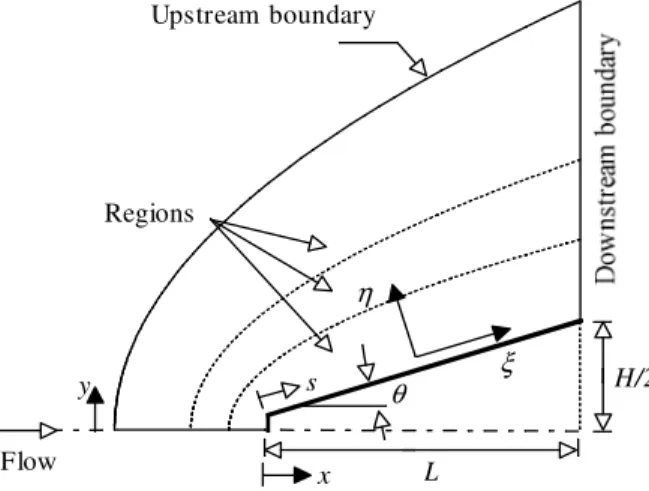
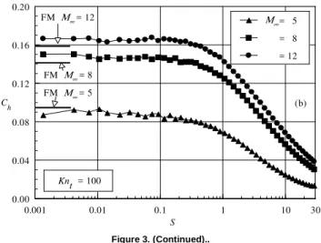
The compressibility effect on the heat transfer coefficient Ch is
plotted in Figs. 3 and 4 for leading edge thickness t/λ∞ of 0.01 and 1, respectively, which correspond to thickness Knudsen number Knt
of 100 and 1. In this set of plots, Figs. 3(a) and 4(a) correspond to the heat transfer coefficient Ch on the front surface as a function of
the dimensionless height Y (≡y/λ∞), measured from the stagnation point up to the shoulder of the wedge, and Figs. 3(b) and 4(b) correspond to the heat transfer coefficient Ch to the afterbody
of 10 (t/λ∞ of 0.1) will not be presented since they are similar to the Knt of 100.
According to Figs. 3 and 4, it is seen that the heat transfer coefficient Ch changes on the front and afterbody surfaces of the
wedge with increasing freestream Mach number. As the freestream Mach number increases from 5 to 12, the kinetic energy of the freestream molecules increases. As a result, the heat flux to the body surface increases. An understanding of this behavior can be gained by Eq. (2). The incident component of the velocity c of the molecules is a function of the freestream Mach number. However, the reflected component of the molecular velocity is not a function of the freestream Mach number. Due to the diffuse reflection model, the reflected component of the molecular velocity is obtained from a Maxwellian distribution that only takes into account for the temperature of the body surface, which has the same value for the freestream Mach number range investigated. It should also be emphasized that the number of molecules colliding with the surface by unit time and unit area, N, which appears in Eq. (2), is the same for the incident and reflected components of the heat transfer coefficient Ch. Nevertheless, N dramatically increases in the front
surface of the leading edges with increasing the freestream Mach number (not shown).
Referring to Figs. 3 and 4, it is also observed that the heat transfer coefficient is sensitive to the leading edge thickness. As would be expected, the blunter (flatter) the leading edge is the lower the heat transfer coefficient along the front surface. A similar behavior is also observed on the afterbody surface where the heat transfer coefficient decreases with increasing the leading edge thickness. Particular attention is paid to the heat transfer coefficient at the vicinity of the shoulder for the bluntest case investigated, Knt
= 1( t/λ∞ = 1). For the Knt= 1 case, the heat transfer coefficient Ch
increases at the vicinity of the shoulder, in contrast to the sharp leading edge cases investigated. This behavior would be also expected since the velocity of the molecules increases at the vicinity of the shoulder on the front surface, where the flow is allowed to expand. In addition, the contribution of the translational energy to the net heat flux varies with the square of the velocity of the molecules, as shown in Eq. (2).
M∞
0.0 0.2 0.4 0.6 0.8 1.0
0.0001 0.001 0.01
Ch
Y
= 5 = 8
= 12 (a) FM Μ∞ = 8
Μ∞
FM Μ∞ = 5 FM Μ∞ = 12
Knt = 100
Figure 3. Heat transfer coefficient Ch along the (a) front surface and (b) the afterbody surface of the wedge as a function of the freestream Mach number for the thickness Knudsen number of 100.
0.00 0.04 0.08 0.12 0.16 0.20
0.001 0.01 0.1 1 10 30
C h
S
= 5 = 8 = 12
(b)
Μ∞
FM Μ∞ = 5 FM Μ∞ = 12
FM Μ∞ = 8
Kn t = 100
Figure 3. (Continued)..
For purpose of comparison, Figs. 3 and 4 display the free molecular flow (FM) limit value for the heat transfer coefficient by assuming free collision flow (Bird, 1994). The values predicted by the free collision flow equations for the heat transfer coefficient Ch
on the front surface are 0.514, 0.810 and 0.916 for freestream Mach number M∞ of 5, 8 and 12, respectively. For the afterbody surface, the FM values are 0.095, 0.142 and 0.159 for M∞ of 5, 8 and 12, respectively. Therefore, it is clearly seen from Fig. 3 that the sharpest leading edge investigated, t/λ∞ = 0.01 case, approaches the free collision flow on the front surface as well as on the afterbody surface at the vicinity of the shoulder. As matter of fact, this is an expected behavior since this leading edge corresponds to a thickness Knudsen number Knt of 100. In contrast, the flow is far from the
free molecular limit for the bluntest leading edge, Knt of 1, as shown
in Fig. 4.
It may be recognized from Fig. 3(b) that the heat transfer coefficient Ch on the afterbody surface at the vicinity of the
flat-face/afterbody junction is above that predicted by the free molecular flow equations. It should be mentioned in this context that this behavior is usually observed on the surface properties at the vicinity of the nose for sharp leading edges such as flat plate, wedge and cone. This is explained by the fact that collision of the oncoming freestream molecules, therefore high-velocity molecules, with the molecules emitted from the body surface will on the average causes at least some of the oncoming molecules to be reflected onto the wedge surface, thereby increasing the heat transfer rate over the free molecular value owing to the increased energy. This result is in contrast to the rarefied flow past blunt leading edge, as shown in Fig. 4(b). For the blunt leading edge, the effect of collisions of the oncoming freestream molecules with those emitted from the surface will be to deflect some of the incident molecules from the surface, thereby reducing the heat transfer rate relative to the free molecular value. As an illustrative example, Vidal and Bartz (1969) observed from their experimental investigations on flat plates and wedges that the heat transfer rate approached the free molecular limit from above whereas those obtained at large wedge angles approached from below. According to them, for the particular conditions on the experiment, a 2-degree wedge angle appeared to be the crossover point where the approach to the free molecular limit was at the level of the free molecular limit. Their wedge flows were produced by pitching the flat-plate model to various compression angles.
Total Drag Coefficient
the surface. The total drag is obtained by the integration of the pressure pw and shear stress τw distributions along the wedge
surface. In an effort to understand the nature of the pressure and shear stress forces acting on the surface of the truncated leading edges, both forces will be also presented in this section.
The pressure pw on the wedge surface is calculated by the sum
of the normal momentum fluxes of both incident and reflected molecules at each time step as follows,
[ ] [ ]
{
}
∑
= +
= +
= N
j j j i j j r r
i
w p p mc mc
p
1
2 2
η
η (3)
M∞
0.0 0.2 0.4 0.6 0.8 1.0
0.001 0.01 0.1 1
C h
Y
= 5 = 8 = 12
(a) FM Μ∞ = 5
Μ∞
FM Μ∞ = 12
FM Μ∞ = 8
Knt = 1
0.00 0.04 0.08 0.12 0.16 0.20
0.001 0.01 0.1 1 10 30
C h
S
= 5 = 8 = 12
(b)
Μ∞
FM Μ∞ = 5 FM Μ∞ = 12
FM Μ∞ = 8
Knt = 1
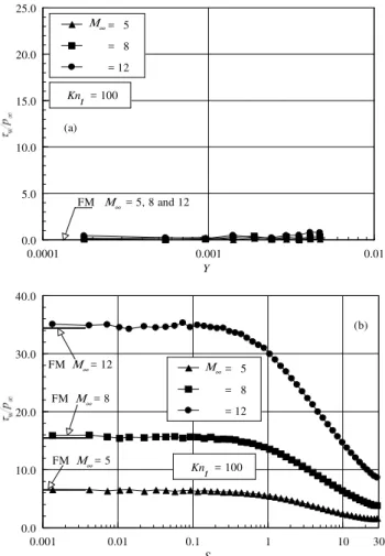
Figure 4. Heat transfer coefficient Ch along the (a) front surface and (b) the afterbody surface of the wedge as a function of the freestream Mach number for the thickness Knudsen number of 1.
where cη is the normal component (η-direction in Fig. 2) of the molecular velocity.
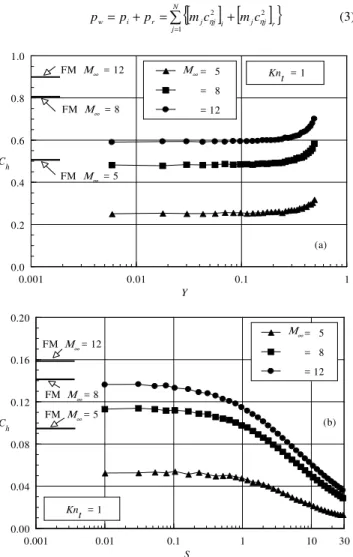
The sensitivity of the wall pressure to variations on the freestream Mach number is demonstrated in Figs. 5 and 6 for cases corresponding to thickness Knudsen number Knt of 100 and 1,
respectively. In this set of diagrams, Figs. 5(a) and 6(a) correspond to the wall pressure, normalized by the freestream pressure p∞, on the front surface as a function of dimensionless height Y, and Figs. 5(b) and 6(b) correspond to the dimensionless wall pressure acting on the afterbody surface of the wedge as a function of the dimensionless arc length S. Plotted along with the computational solutions for dimensionless wall pressure is the wall pressure limit predicted by the free molecular (FM) flow equations.
Referring to Figs. 5 and 6, it is noted that the pressure basically present a constant value along the front surface, and the constant
value increases with increasing the freestream Mach number. It can also be seen that the front surface experiences a remarkable pressure compared to the freestream pressure; it is one order of magnitude larger than the freestream pressure for the M∞ = 5 case, and two orders of magnitude larger than the freestream pressure for the other two freestream Mach number cases investigated. It should be mentioned in this context that the large amount of kinetic energy presented in a hypersonic freestream is converted by molecular collisions into high thermal energy surrounding the body and by flow work into increased pressure. In this way, the region at the vicinity of the front surface is a zone of strong compression.
Similar to the pressure on the front surface, the pressure on the afterbody surface increases with a freestream Mach number rise. It is also apparent from Figs. 5 and 6 that the pressure on the afterbody surface is one order of magnitude smaller than that on the front surface. Furthermore, as the leading edge thickness increases, the nose of the leading edge becomes blunter and a rather different flow behavior is observed, in the sense that the wall pressure for the Knt =
1 (t/λ∞ = 1) case does not display the same structure as that presented by the Knt = 100.
M∞
0 50 100 150 200 250
0.0001 0.001 0.01
Y
= 5 = 8 = 12
(a) FM Μ∞ = 8
Μ∞
FM Μ∞ = 5 FM Μ∞ = 12
Kn t = 100
0.0 5.0 10.0 15.0 20.0 25.0 30.0
0.001 0.01 0.1 1 10 30
S
= 5 = 8 = 12
(b)
Μ∞
FM Μ∞ = 5 FM Μ∞ = 12
FM Μ∞ = 8
Knt = 100
Figure 5. Dimensionless wall pressure (pw/p∞∞∞∞) along the (a) front surface and (b) the afterbody surface of the wedge as a function of the freestream Mach number for the thickness Knudsen number of 100.
The difference between the pressure distribution along the surface for Knt = 100 case from Knt=1 case is explained by the fact
that the leading edge defined for Knt = 100 behaves aerodynamically
like a sharp leading edge. In contrast, the leading edge defined for Knt = 1 behaves aerodynamically like a blunt leading edge. The
similar to the number flux distribution, i.e., the number of molecules colliding by unit time and unit area. For Knt = 100 case, the number
flux is close to the free-molecular value at the vicinity of the shoulder, then there is a sharp increase in the number flux which reaches a maximum at about one freestream mean free path from the shoulder. Therefore, the maximum value for Cp is firmly established
by the maximum point attained by the number flux. On the other hand, for Knt = 1 case that behaves like a bunt body, the number
flux is maximum at the shoulder and then drops off along the afterbody surface. It is important to mention that the pressure distribution is directly related to the number flux, as shown in Eq. (3).
According to Fig. 5, the wall pressure reaches the limit values predicted by the free molecular flow as expected, since for the t/λ∞
= 0.01 case the overall Knudsen number is Knt = 100, as mentioned
earlier. In contrast, according to Fig. 6, the pressure on both front and afterbody surfaces is far from the limit value predicted by the free molecular flow equations (Bird, 1994). It is also seen that the wall pressure on the afterbody surface is one order of magnitude smaller than that on the front surface.
The shear stress τw on the body surface is calculated by the sum
of the tangential momentum fluxes of both incident and reflected molecules at each time step as follows,
[ ] [ ]
{
}
∑
= +
= +
= N
j j j i j jr r
i
w mc mc
1
2 2
ξ ξ τ
τ
τ (4)
where cξ is the tangential component (ξ-direction in Fig. 2) of the molecular velocity.
For the diffuse reflection model imposed for the gas-surface interaction, reflected molecules have a tangential moment equal to zero, since the molecules essentially lose, on average, their tangential velocity component. In this fashion, the second term on the right-hand side of Eq. (4) disappears, and the wall shear stress τw
reduces to the following expression,
M∞
0 50 100 150 200 250
0.001 0.01 0.1 1
Y
= 5 = 8 = 12
(a) FM Μ∞ = 8
Μ∞
FM Μ∞ = 5 FM Μ∞ = 12
Knt = 1
Figure 6. Dimensionless wall pressure (pw/p∞∞∞∞) along the (a) front surface and (b) the afterbody surface of the wedge as a function of the freestream Mach number for the thickness Knudsen number of 1.
0.0 5.0 10.0 15.0 20.0 25.0 30.0
0.001 0.01 0.1 1 10 30
S
= 5 = 8 = 12
(b)
Μ∞
FM Μ∞ = 5 FM Μ∞ = 12
FM Μ∞ = 8
Kn t = 1
Figure 6. (Continued).
[ ]
{
}
∑
= =
= N
j j ji i
w mc
1 2
ξ τ
τ (5)
Distributions of shear stress τw, normalized by the freestream
pressure p∞, along the wedge surface are displayed in Figs. 7 and 8 parameterized by the freestream Mach number. Figures 7(a) and 8(a) illustrate the dimensionless shear stress on the front surface for Knt of 100 and 1, respectively, while Figs. 7(b) and 8(b) depict the
dimensionless shear stress on the afterbody surface for the same two cases.
As seen from Figs. 7(a) and 8(a), the distributions of the dimensionless shear stress τw/p∞ on the front surface are nearly
identical for the cases investigated. It is zero at the stagnation point and increases along the front surface up to the shoulder of the wedge. Furthermore, the value for τw/p∞ significantly increases near
the shoulder of the wedge with increasing the thickness of the leading edge. The trend of the distributions on the front surface is as expected since the velocity of the molecules increases in the vicinity of the shoulder due to the flow expansion. As a result, the tangent momentum of the molecules increases in this region, even though the number of molecules impinging on the front surface decreases in the vicinity of the shoulder (not shown) for the same M∞.
M∞
0.0 5.0 10.0 15.0 20.0 25.0
0.0001 0.001 0.01
Y
= 5 = 8 = 12
(a)
Μ∞
FM Μ∞ = 5, 8 and 12
Kn t = 100
0.0 10.0 20.0 30.0 40.0
0.001 0.01 0.1 1 10 30
S
= 5 = 8 = 12
(b)
Μ∞
FM Μ∞ = 5 FM Μ∞ = 8 FM Μ∞ = 12
Knt = 100
Figure 7. Dimensionless wall shear stress (ττττw/p∞∞∞∞) along the (a) front surface and (b) the afterbody surface of the wedge as a function of the freestream Mach number for the thickness Knudsen number of 100.
Comparison of the computed wall shear stress with that predicted by considering free collision flow shows that the values are very close one to each other for the Knt = 100 case, as displayed
in Fig. 7. As a reference, the FM values are equal to zero along the front surface for M∞ of 5, 8 and 12. Along the afterbody surface the FM values are 6.4, 15.5 and 34.5 for freestream Mach number of 5, 8 and 12, respectively.
The total drag coefficient Cd is defined as being,
H M
p F H V F
Cd 2
2 1 2 2 1
∞ ∞ ∞
∞ = =
γ
ρ (6)
where F is the resultant force acting on the body surface, γ is the specific heat ratio and H is the height at the matching point common to the leading edges (see Fig. 1).
The resultant force acting on the wedge was obtained by the integration of the pressure pw and shear stress τw distributions from
the stagnation point of the leading edge to the station L that corresponds to the tangent point common to all wedges (see Fig. 1). It is worthwhile mentioning that the values for the total drag coefficient were obtained by assuming the shapes acting as leading edges. Consequently, no base pressure effects were taken into account on the calculations. The DSMC results for total drag coefficient are presented as total drag coefficient Cd and its
components of pressure drag coefficient Cpd and skin friction drag
coefficient Cfd.
M∞
0.0 5.0 10.0 15.0 20.0 25.0
0.001 0.01 0.1 1
Y
= 5 = 8 = 12
(a)
Μ∞
FM Μ∞ = 5, 8 and 12
Knt = 1
0.0 10.0 20.0 30.0 40.0
0.001 0.01 0.1 1 10 30
S
= 5 = 8 = 12
(b) Μ∞
FM Μ∞ = 5 FM Μ∞ = 8 FM Μ∞ = 12
Knt = 1
Figure 8. Dimensionless wall shear stress (ττττw/p∞∞∞∞) along the (a) front surface and (b) the afterbody surface of the wedge as a function of the freestream Mach number for the thickness Knudsen number of 1.
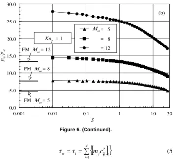
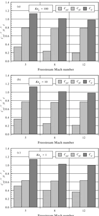
The impact of the compressibility on the total drag coefficient is depicts on Figs. 9(a-c) for leading edges corresponding to Knt of
100, 10 and 1, respectively. According to this set of figures, it should be noticed that as the leading edge becomes blunt (Knt
→
1) the contribution of the pressure drag coefficient Cpd to the total drag
coefficient increases and the contribution of the skin friction drag coefficient Cfd decreases. As the net effect on total drag coefficient
depends on these two opposite behaviors, hence no appreciable changes are observed in the total drag coefficient for the leading edge thickness cases investigated, by considering the same freestream Mach number. As a reference, for freestream Mach number of 5, the pressure drag is 30% and 44.3% of the total drag for the leading edges defined by Knt of 100 and 1, respectively. On
the other hand, the skin friction contribution decreases from 70% to 55.7% for the same cases. This behavior appears to be fully explained through the changes in pressure and shear stress shown from Figs. 5 to 8. Note that on the front surface, for the same freestream Mach number, the wall pressure slightly decreases as the leading edge thickness increases, while it tends to increase on the afterbody surface of the wedge. In contrast, the shear stress basically has no contribution on the front surface, however it decreases on the afterbody surface.
stress significantly increase with freestream Mach number, as depicted from Figs. 5 to 8. Equation (6) provides the necessary assistance in order to understand this behavior. The numerator of Eq. (6) grows with wall pressure and shear stress, while the denominator (∝M∞2) increases faster than the numerator and results in a total drag coefficient decrease.
(c)
5 8 12
0.0 0.2 0.4 0.6 0.8 1.0 1.2 1.4
Freestream Mach number
Cpd Cfd Cd
(a)
Knt = 100
(c)
5 8 12
0.0 0.2 0.4 0.6 0.8 1.0 1.2 1.4
Freestream Mach number
Cpd Cfd Cd
(b)
Knt = 10
(c)
5 8 12
0.0 0.2 0.4 0.6 0.8 1.0 1.2 1.4
Freestream Mach number
Cpd Cfd Cd
(c)
Knt = 1
Figure 9. Pressure drag Cpd, skin friction drag Cfd and total drag Cd coefficients as a function of the freestream Mach number for thickness Knudsen number Knt of (a) 100, (b) 10 and (c) 1.
Comparison of Results with Experimental Data
In this section, the DSMC results for pressure acting on, and heat transfer to the wedge surface are compared to the available
experimental data. The experimental data of Vidal and Bartz (1966 and 1969) used two flat-plate models, one small and the other large, in experimental wedge research. The wedge flows were produced by varying the inclination of the plates between 2 and 40 degrees with respect to the freestream direction. The small-scale flat plate model was designed to investigate the heat transfer in the vicinity of the leading edge, whereas the large-scale model to investigate the wall pressure. The leading edge models were flat-faced with a thickness estimated to be 1.27x10⁻⁴m (0.005 in).
0.0 2.0 4.0 6.0 8.0
0.0001 0.001 0.01 0.1 1 10 100
Re s/γ M∞
2
C *cosθ
Knt = 100 Vidal and Bartz (1969)
Chow and Eilers (1968) 8
M∞= 5
12
FM Limit M∞= 12
8 5
(a)
0.0 2.0 4.0 6.0 8.0
0.0001 0.001 0.01 0.1 1 10 100
Re s/γ M∞
2
C *cosθ
Knt = 1 Vidal and Bartz (1969)
Chow and Eilers (1968) 8
M∞= 5
12
FM Limit M
∞= 12
8 5
(b)
Figure 10. Comparison of normalized pressure along the afterbody surface of the wedge for leading edge cases corresponding thickness Knudsen number of (a) 100 and (b) of 1.
Figures 10(a) and 10(b) show a comparison of the pressure on the wedge surface for two leading edge cases corresponding to Knt
of 100 and 1, respectively. In this set of figures, the vertical axis is the surface pressure normalized by the Newton-Buseman approximation for wedge pressure, and the abscissa is the normalized distance used by Vidal and Bartz (1969). The quantity C* is the modified Chapman-Rubesin constant, which is defined by
the following expression,
* * *
T T
C ∞
∞ =
µ µ
(7)
where µ* is the viscosity at the reference temperature T* given by,
o w *
T T T
T
2 1 6 1+ = ∞
For comparison purpose, the surface pressure obtained from the theory proposed by Chow and Eilers (1968) is also shown in Fig. 10.
Referring to Figs. 10(a) and 10(b), the experimental data of Vidal and Bartz (1969) are for wedges with half angle of 10 deg, freestream Mach numbers of 19 (square symbols) and 20.7 (circle symbols), which correspond to freestream unit Reynolds numbers of 11000/m and 85000/m, respectively. It is seen from these figures that the DSMC results tend to the experimental data far from the nose of the leading edge, where the bluntness effects are no longer important. Also, it may be recognized from these figures that the DSMC results tend to those predicted by experimental data with the freestream Mach number rise. This behavior may be explained by the Mach number independence principle in that the wall pressure and drag reach a limit value by increasing the freestream Mach number.
0 .0 0 .2 0 .4 0 .6 0 .8 1 .0
0 .00 1 0 .0 1 0 .1 1 1 0
R e s/γ M∞
2 C
*co sθ
Vid al an d Bar tz ( 1 96 6 )
M∞= 5
K n t = 1 8 1 2
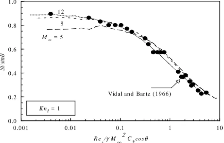
Figure 11. Comparison of normalized heat transfer flux along the afterbody surface of the wedge for leading edge case corresponding thickness Knudsen number of 1.
It should be mentioned that the surface measurements presented by Vidal and Bartz (1969), supposed to cover the transition from the strong interaction boundary-layer regime to the limit case of a free molecular flow, did not predict the pressure closer to the shoulder of the wedge when compared to the DSMC results. They expected that the surface pressure would approach to the free-molecular limit in the immediate vicinity of the leading edge. The difficulty arises from the complication of installing pressure taps very close to the nose of the leading edge. Furthermore, in low-density flows, the true pressure on a surface can be significantly different from that measured in orifice cavities or pressure holes, because of the increase in the effect of molecule-surface collisions, the so-called orifice effect (Potter et al., 1966). In addition, experimental measurements in the low-density conditions must detect extremely low pressure that require special instrumentation.
Figure 11 presents the comparison for the heat transfer to the afterbody surface of the wedge for Knt= 1 case. In the figure, the
Stanton number St is plotted as a function of the Reynolds number Re. It can be seen that the DSMC results for the heat flux follow the same trend shown by the experimental data. Nevertheless, despite the good agreement of the DSMC results for the Knt= 1 case, which
corresponds to the leading edge thickness t/λ∞ = 1, the experimental data were obtained for a wedge with a leading edge thickness of 1.27x10⁻⁴m (0.005 in), and no further conclusion can be drawn,
because it was not possible to identify the freestream conditions related to this leading-edge thickness as well as to calculate the mean free path from the various freestream conditions used by Vidal and Bartz (1966 and 1969).
Concluding Remarks
This study applies the Direct Simulation Monte Carlo method to investigate rarefied gas over truncated wedges. Effects of air speed on the heat transfer coefficient, wall pressure, wall shear stress and drag coefficient for representative ranges of parameters are examined. The freestream Mach number is varied from 5 to 12, and the Knudsen number, based on the front surface thickness of the leading edges, ranges between 1 and 100. Cases considered in this study cover the hypersonic flow in the transitional and free molecular flow regimes.
Performance results for leading edge thickness t/λ∞ of 0.01, which corresponds to thickness Knudsen number of 100, indicated that the flow approaches the free molecular flow at the vicinity of the front surface, for the freestream Mach number considered. Substantial changes in the aerodynamic surface quantities were observed as the leading edge thickness increased. It was found that the total drag coefficient presented almost the same values for a fixed freestream Mach number. However, as expected it decreased as the freestream Mach number increased.
Results indicated that, with the size of the models being tested in hypersonic tunnels, significant effects on aerodynamic surface quantities due to leading edge thickness are possible even with models whose leading edges are generally considered as being aerodynamically sharp.
Appendix
This section focuses on the analysis of the influence of the cell size and the number of molecules per computational cell on the surface properties in order to achieve grid independent solutions.
In the DSMC method, a computational mesh has to be constructed to form a reference for selecting collision partners and for sampling and averaging the macroscopic flowfield properties. In order to accurately model the collision process, the cell size of a computational cell should be on the order of one-third of the local mean free path in the direction of primary gradients (Alexander et. al., 1998 and 2000). Close to the body surface, cell spacing normal to the body should also to be of the order of a third of the local mean free path. If the cell size near the body surface is too large, then energetic molecules at the far edge of the cell are able to transmit momentum and energy to molecules immediately adjacent to the body surface. This leads to overprediction of both the surface heat flux and the aerodynamic forces on the body that would occur in the real gas (Haas and Fallavollita, 1994). Hence, heat transfer coefficient and pressure coefficient are used as the representative parameters for the grid sensitivity study. In addition, the analysis presented in this section is limited to the leading edge case corresponding to Knt = 1. The same procedure was employed for the
other cases. Therefore, they will not be shown.
Effect of Grid Variation
The effect of altering the size of the computational cells is investigated for a series of three simulations with grids of 50 (coarse), 100 (standard) and 150 (fine) cells in the ξ-direction and 60 cells in the η-direction. From the total number of cells in the ξ -direction, 30% are located along the frontal surface and 70% distributed along the afterbody surface. Each grid was made up of non-uniform cell spacing in both directions.
The effect of changing the number of cells in the ξ-direction is illustrated in Figs. A(1) and B(1) for the frontal and afterbody surfaces, respectively, as it impacts the calculated heat transfer and pressure coefficients. The comparison shows that the calculated results are rather insensitive to the range of cell spacing considered.
In analogous fashion, an examination was made in the η -direction. The sensitivity of the heat transfer and pressure coefficients to cell size variations in the η-direction is displayed in Figs. A(2) and B(2) for frontal and afterbody surfaces, respectively. In this set of figures, a new series of three simulations with grid of 100 cells in the ξ-direction and 30 (coarse), 60 (standard) and 90 (fine) cells in the η-direction is compared. The cell spacing in both directions is again non-uniform.
0.0 0.5 1.0 1.5 2.0 2.5
0.001 0.01 0.1 1
Y
C h
50 X 60 100 X 60 150 X 60
ξ η
C p
(1)
0.0 0.5 1.0 1.5 2.0 2.5
0.001 0.01 0.1 1
Y
C p
C h
ξ η
100 X 30 100 X 60 100 X 90
(2)
Figure A. Effect of altering the cell size along the (1) .ξξξξ-direction and (2) ηηηη -direction and (3) the effect of altering the number of molecules on pressure and heat transfer coefficients related to the frontal surface.
0.0 0.5 1.0 1.5 2.0 2.5
0.001 0.01 0.1 1
Y
C h
104,000 Mols. 190,000 Mols. 283,000 Mols.
C p
(3)
Figure A (Continued)..
According to Figs. A(2) and B(2), the results for the three grids are approximately the same, indicating that the standard grid, 100x60 cells, is essentially grid independent. For the standard case, the cell size in the η-direction is always less than the local mean free path length in the vicinity of the surface.
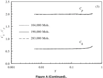
Effect of Number of Molecules
A similar examination was made for the number of molecules. The sensitivity of heat transfer and pressure coefficients to variations on the number of molecules is demonstrated in Figs. A(3) and B(3) for frontal and afterbody surfaces, respectively. The standard grid, 100x60 cells, corresponds to a total of 190,000 molecules. Two new cases using the same grid were investigated. These new cases correspond to, on average, 104,000 and 283,000 molecules in the entire computational domain. Referring to Figs. A(3) and B(3), It is seen that the standard grid with a total of 190,000 molecules is enough for the computation of the aerodynamic surface quantities on the truncated leading edges.
0.0 0.1 0.2 0.3
0.01 0.1 1 10 30
S
C h
50 X 60 100 X 60 150 X 60
ξ η
C p
(1)
0.0 0.1 0.2 0.3
0.01 0.1 1 10 30
S
C p
C h
ξ η
100 X 30 100 X 60 100 X 90
(2)
0.0 0.1 0.2 0.3
0.01 0.1 1 10 30
S
C h
104,000 Mols. 190,000 Mols. 283,000 Mols.
C p
(3)
Figure B. (Continued).
References
Alexander, F. J., Garcia, A. L., and, Alder, B. J., 1998, “Cell Size Dependence of Transport Coefficient in Stochastic Particle Algorithms”, Physics of Fluids, Vol. 10, No. 6, pp. 1540-1542.
Alexander, F. J., Garcia, A. L., and, Alder, B. J., 2000, “Erratum: Cell Size Dependence of Transport Coefficient is Stochastic Particle Algorithms”, Physics of Fluids, Vol. 12, No. 3, pp. 731-731.
Anderson, J. L., 1990, “Tethered Aerothermodynamic Research for Hypersonic Waveriders”, Proceedings of the 1st International Hypersonic Waverider Symposium, Univ. of Maryland, College Park, MD.
Bird, G. A., 1981, “Monte Carlo Simulation in an Engineering Context”, Progress in Astronautics and Aeronautics: Rarefied gas Dynamics, Ed. Sam S. Fisher, Vol. 74, part I, AIAA New York, pp. 239-255.
Bird, G. A., 1989, “Perception of Numerical Method in Rarefied Gasdynamics”, Rarefied gas Dynamics: Theoretical and Computational Techniques, Eds. E. P. Muntz, and D. P. Weaver and D. H. Capbell, Vol. 118, Progress in Astronautics and Aeronautics, AIAA, New York, pp. 374-395.
Bird, G. A., 1994, “Molecular Gas Dynamics and the Direct Simulation of Gas Flows”, 1st edition, Oxford University Press, Oxford, England, UK., 458p
Borgnakke, C. and Larsen, P. S., 1975, “Statistical Collision Model for Monte Carlo Simulation of Polyatomic Gas Mixture”, Journal of computational Physics, Vol. 18, No. 4, pp. 405-420.
Chow, W. L., and Eilers, R. E., 1968, “Hypersonic Low-Density Flow past Slender Wedges”, AIAA Journal, Vol. 6, No. 1, pp.177-179.
Garcia, A. L., and, Wagner, W., 2000, “Time Step Truncation Error in Direct Simulation Monte Carlo”, Physics of Fluids, Vol. 12, No. 10, pp. 2621-2633.
Graves, R. E. and Argrow, B. M., 2001, “Aerodynamic Performance of an Osculating-Cones Waverider at High Altitudes”, 35th AIAA Thermophysics Conference, Paper AIAA 2001-2960, Anaheim, CA.
Guo, K. and Liaw, G.-S., 2001, “A Review: Boundary Conditions for the DSMC Method”, Proceedings of the 35th AIAA Thermophysics Conference, AIAA Paper 2001-2953, Anaheim, CA, 11-14 June.
Haas, B, L., and Fallavollita, M. A., 1994, “Flow Resolution and Domain Influence in Rarefied Hypersonic Blunt-Body Flows”, Journal of Thermophysics and Heat Transfer, Vol. 8, No. 4, pp. 751-757.
Hadjiconstantinou, N. G., 2000, “Analysis of Discretization in the Direct Simulation Monte Carlo”, Physics of Fluids, Vol. 12, No. 10, pp. 2634-2638. Nonweiler, T. R. F., 1959, “Aerodynamic Problems of Manned Space Vehicles”, Journal of the Royal Aeronautical Society, Vol. 63, Sept, pp. 521-528.
Potter, J. L., Kinslow, M. and Boylan, D. E., 1966, “An Influence of the Orifice on Measured Pressures in Rarefied Flow”, Rarefied Gas Dynamics, edited by J. H. de Leeuw, Academic Press, New York, Vol. II, pp. 175-194.
Potter, J. L. and Rockaway, J. K., 1994, “Aerodynamic Optimization for HypersonicFlight at Very High Altitudes”, Rarefied Gas Dynamics: Space Sciences and Engineering, Progess in Astronautics and Aeronautics, vol. 160, Ed. B. D. Shizgal and D. P. Weaver, pp. 296-307.
Rault, D. F. G., 1994, “Aerodynamic Characteristics of a Hypersonic Viscous Optimized Waverider at High Altitude”, Journal of Spacecraft and Rockets, Vol. 31, No. 5, pp. 719-727.
Santos, W. F. N., 2002, “Truncated Leading Edge Effects on Flowfield Structure of a Wedge in Low Density Hypersonic Flight Speed”, Proceedings of the 9th Brazilian Congress of Thermal Engineering and Sciences, Paper CIT02-0879, Caxambu, MG, Brazil.
Santos, W. F. N., 2005, “Flat-Faced Leading Edge Effect in Low Density Hypersonic Wedge Flow”, Journal of Spacecraft and Rockets, Vol. 42, No. 1, pp.22-29.
Shvets, A. I., Voronin, V. I., Blankson, I. M., Khikine, V. And Thomas, L., 2005, “On Waverider Performance with Hypersonic Flight Speed and High Altitudes”, 43rd AIAA Aerospace Sciences Meeting and Exhibit, AIAA Paper 2005-0512, Reno, NV.
Vidal, R. J. and Bartz, J. A., 1966, “Experimental Studies of Low-Density Effects in Hypersonic Wedge Flows”, Rarefied Gas Dynamics, edited by J. H. de Leeuw, Academic Press, New York, Vol. I, pp. 467-486.