Article
J. Braz. Chem. Soc., Vol. 26, No. 9, 1848-1860, 2015. Printed in Brazil - ©2015 Sociedade Brasileira de Química 0103 - 5053 $6.00+0.00
A
*e-mail: [email protected]
Potentiometric Titration and Out-Of-Equilibrium pH Response of the
Biotite-Water System
Vicente R. Almeida,*,a,b Bruno Szpoganicza and Steeve Bonnevilleb
aDepartamento de Química, Universidade Federal de Santa Catarina,
88040-900 Florianópolis-SC, Brazil
bBiogéochimie et Modélisation du Système Terre, Départment des Sciences de la Terre et de
l’Environnement, Université Libre de Bruxelles, 1050 Brussels, Belgium
Minerals in soils contribute significantly to the capacity of soils to buffer pH disturbance. In this paper, we present the pH buffering capacity of a common soil phyllosilicate mineral, biotite. We performed equilibrium potentiometric titrations and we also monitored the pH response kinetics of the mineral-water system in order to develop an out-of-equilibrium model able to capture the interactions between minerals and the surrounding aqueous fluid. During titrations, after each addition of titrant solution from pH 11 to ca. 3, the pH response patterns were monitored over time until reaching a pseudo-equilibrium pH value. Based on the potentiometric dataset Best7, equilibrium calculations were performed to obtain the concentrations and the equilibrium protonation constants of each deprotonable component that fit best our titration curve. In parallel, the out-of-equilibrium pH responses over time at each point of the titration were used in a simple first-order kinetic approach that allow for the determination of “slow” proton exchange [H+
ex]t0 (mol L
-1) and the associated rate constants for the exchange reactions, k (s-1). Our results show a maximum in “slow” proton exchange [H+
ex]t0 associated to a minimal value of k at pH < 5 while at neutral and basic pH exhibits the opposite, i.e., fast rate constant for a minimum value of the “slow” proton exchange. Expressing the observed “slow” proton exchange processes in terms of entropy production, our result demonstrate that the maximum resilience stability of biotite-water system to pH perturbation is in acidic pH, probably due to the consumption of proton associated with biotite dissolution reactions.
Keywords: potentiometric titrations, biotite, linear out-of-equilibrium thermodynamics, soils
Introduction
In recent decades, capturing landscape and environmental complexity has been a challenge for
sciences.1,2 Furthermore, human activities deeply affect the
earth system and the biosphere. In particular the interactions between natural water and soils deserve careful attention when facing disturbances. As first approach, it appears reasonable to propose an epistemological standing point based on differences, which can be understood as the main
feature of complex heterogeneity.3 The concept of difference
observation has enormous utility in science,3,4 and in the
case of chemistry, one can point out that difference is at
the basis of thermodynamics and change of state.5 Physical
chemistry can provide powerful tools to explore and
understand landscape evolution and complexity.5-7 Here,
we propose not only to study the relations between water and minerals in soils but also to explore the stability of this heterogeneous system to pH perturbations, a master variable in soil chemistry. Indeed, soil pH affect a wide range of soil chemical and biological properties (i.e., vegetation assemblages, root nutrient uptake, diversity and activity of soil microorganisms, as well as, the mobility and
toxicity of pollutants for instance).8-13
as a rock-forming mineral of granitic rocks and as such
it represents up to 7% of the exposed continental crust.14
Biotite alteration in soils is a major source of K, Mg and
Fe for soil biota, vegetation and ultimately groundwater.15
A large body of literature has been dedicated to
equilibrium potentiometric titrations of minerals,12,13,16 in
which titration curves are constructed by the compilation of pH measurements at equilibrium after each addition of titrants. However, the pH response and kinetic behavior of the disturbed mineral-water system convey a wealth of information on system stability facing pH perturbations, yet few studies have been dedicated to out-of-equilibrium
behavior of minerals.12,13 The same knowledge gaps can
be stated for the organic and biogeochemical matrix of soils such as organic matter and/or microorganisms where literature on equilibrium potentiometric titration is relatively rich but their response to pH perturbation has
been far less studied.9,12,16-20
In this study, we present a simple approach that covers both out-of-equilibrium response patterns of disturbed pH states and equilibrium states of water-biotite system, all within a single method of kinetically-resolved potentiometric titration and data treatment. It is also important to point out the accessible, environmentally-friendly and cost-efficient character of this electrochemical method, and also the pedagogical relevance of our approach, in which a transdisciplinar view is proposed, in this case to study soil/mineral
complexity.1-4,10,21,22
Experimental
Mineral sample
The biotite originated from Moen, Norway, was purchased from Krantz Company. The bulk chemical composition of the biotite was determined in a previous
study,23 by electron microprobe analyser (Cameca SX50)
to be K0.92 Na0.02 (interlayer) Mg0.76 Mn0.05 Fe1.61 Al0.23
(octahedral sheet) Al1.26 Si2.74 (tetrahedral sheet) (OH2) O10).
The biotite was crushed using a mortar and the fraction < 300 µm was used for the experiments.
Kinetically-resolved potentiometric titrations
All experiments and blanks were performed in triplicate in a 100 mL glass reactor connected to a thermostated bath at 25.0 °C. The reactor was kept under constant
water-saturared N2 gas flow and vigourous magnetic bar
stirring and also ultra-pure degassed water was used in all experiments. The accuracy of the combined glass
electrode was tested with a blank titration of a 40 mL
solution of 0.0099 mol L-1 HCl (0.1 mol L-1 KCl) by a
titrant solution of 0.1163 mol L-1 CO
2-free NaOH. The
measured potential values were converted to pH using
(–log [H+]) versus volume
titrant theoretical values calculated
with Best7 software,6,7 resulting in a potential versus
pH slope of 99.5% of the Nernst constant at 25.0 °C
(ca. –59.1 mV per pH unit).
The biotite sample, 103 mg, was firstly suspended in
a 40 mL solution of 0.1 mol L-1 KCl and let to equilibrate
for 1 h before titration. At the end of the equilibration period, the pH was stabilized at 9.3 which is in agreement
with the pH range (9.2 to 10) reported in Bray et al.,18
for the same biotite after a 24 h of equilibration period. The pH of the biotite suspension was then raised to
ca. 11 by adding 0.4 mL of a 0.1163 mol L-1 CO
2-free NaOH solution. The titration then proceed with precise
0.1 mL additions of a 0.1019 mol L-1 HCl solution using
a precision (0.01 mL) manual burette(Gilmont; 2 mL).
Following each titrant addition, the pH was monitored regularly at 0, 15, 30, 60, 120, 240, 480 and 960 s. The
final pH values (pHfinal or pHeq), which are the same, see
modeling section (Figure 1 and Figure 2) for each titrant addition were used to construct the potentiometric titration curves and equilibrium calculations while the kinetic pH-response after each titrant addition was the basis for our out-of-equilibrium kinetic model.
Results and Discussion
Figure 1 shows the titration curves obtained for
CO2-free water (blank), centrifuged solution from 1 h
water-equilibrated biotite, the 0-300 µm size fraction biotite-water suspension and the corresponding Best7 model calculation. For the titrations curves in Figure 1, the pH values were registered when the systems show minimal or no pH variations, hence reaching
pseudo-equilibrium (i.e., pHfinal, which is defined as pHeq). A steep
pH variation can be observed for the blank titration and also for the centrifuged solution of 1 h water-equilibrated
biotite, however with a slightly lower slope of pH versus
volume added. For the biotite-water suspension, the titration
curves is much “flatter”, and a larger amount of H+ has
to be added to induce pH changes, meaning that the pH buffering capacity is much larger in the heterogeneous biotite suspension than in both fluid titrations. Note that the titration curve of the centrifuged solution of 1 h water-equilibrated biotite, is very close to the blank titration
meaning that the H+ exchange of hydrolysis reactions
of cations potentially dissolved from biotite is small as
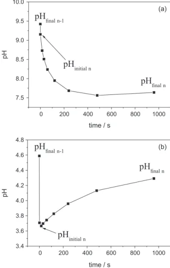
Figure 2 illustrates the pH response over time of the biotite-water system at selected basic and acid pH conditions. Immediately after the titrant addition (from 0 to a maximum of 30 s, depending on the titration point n) the measured pH value drops strongly from the pH value of
the previous titraton point (pHfinal n-1 = pHeq n-1) to the initial
pH value (pHinitial n= pHeq n) of the kinetically measurable
first order “slow” proton exchange.
Note that we do not consider the very initial time pH drop in our kinetical approach as it is probably the result of the diffusion of the titrant into the reactor and the response time of the electrode to the new chemical conditions.
pHinitialn is measured between few seconds and 30 s after
titrant addition. Here, we focus our kinetic approach on
the “slow” exchange pH patterns (from pHinitial n to pHfinal n
in Figures 2a and 2b) that reflect biotite-fluids reactions involving protons. As can be seen in Figure 2a, at basic pH conditions the “slow” proton exchange drives the system (water-biotite) to lower pH, indicating an increase in the proton concentration in the aqueous phase, due most probably to the added acid titrant in the biotite-water system (this pH decrease is slower than in the blank titrations possibly indicating an influence of the biotite in the proton homogenization). In contrast, in acidic pH conditions (Figure 2b), the “slow” proton exchange reactions are probably due to the protonation of biotite conjugate bases, and consumes significant proton amounts from the aqueous phase, thus increasing the pH (see next sections). The
difference between initial pHinitial n and pHfinal n (measured
960 s after titrant addition) can vary significantly from less than 0.01 pH units to ca. 1.5 depending on the pH condition along the pH studied range as illustrated in Figure 3.
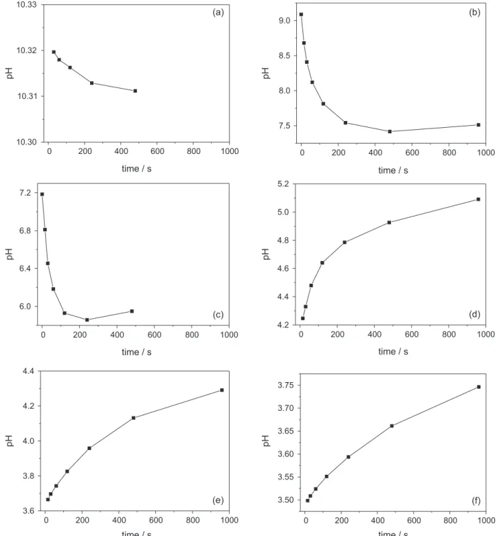
Figure 3 shows the pH variations due to “slow” proton exchange over the studied pH range. In basic conditions (Figures 3a, 3b and 3c), the measured pH tends to decrease and the opposite is observed at acidic conditions (Figures 3d, 3e and 3f). The data from the “slow” pH variations, as presented in Figure 3, was used to establish the first-order kinetics for “slow” proton exchange (see modeling, it will be more discussed in Figure 6).
Modeling of biotite-water system
In this section, we show (i) the potentiometric
equilibrium calculations based on the classical titration
curve using the Best7 software, (ii) a new kinetic framework
to interpret the perturbation pH-response of the biotite-water
system across the pH 3-11 range and (iii) the calculation
of the “slow” proton exchange entropy production as the thermodynamical stability parameter to represent the biotite-water system responses to pH perturbation.
Figure 1. Potentiometric titration curve of the biotite (0-300 µm size fraction), the 1 h biotite-equilibrated solution (collected after 40 min centrifugation at 5000 rpm) and of the CO2-free water. The calculated biotite (0-300 µm) titration curve was performed using Best7 software with small resulting goodness of the fit σfit < 0.03.6
Figure 2. Experimental pH-response from a titration point (pHfinaln−1) to
the next pseudo-equilibration state (pHfinal n = pHeq) after titrant addition
Equilibrium approach
The Best7 software used to fit the equilibrium potentiometric titration curves is a formula translating system (FORTRAN) program currently employed to determine stability constants of chemical component species and related
concentrations in simple or complex aqueous systems.6,7,24
It is essentially based on mass balance calculations using the volume of standard titrant added to the system at all points of the titration. Best7 routines treat the pH (–log
[H+]) as a variable and refine the equilibrium constants and
component concentrations (calculation input) in order to
minimize the error, σfit,
6 between the calculated model and
experimental data (pHfinal n or pHeq, which are the same) of the
titration curve. The first step of our modeling approach is the
calculation of the amount of moles (Ci) and the associated
stability constants (βj) of suggested components, i, and
their related species, j, of the biotite system.6,7 Here, we
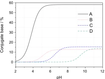
propose a simple component/species model comprised by four sequential component protonation reactions along the studied pH range. The components were named as A, B, C and D (see discussion section for putative sites in biotite) and their respective monoprotic equilibrium constants rank such that βH+A > βH+B > βH+C > βH+D meaning strongest acidity for
conjugate acid H+A and weakest for H+D species. We define
A (not bolded) as the conjugate base species of component A
(bolded), and the same for components B, C and D (Figure 4)
and conjugate bases B, C and D, such as:
H+ + A ⇄ H+A (1)
with
(2)
The program Best7 solves the following equation:
(3)
where Ti is the total concentration of component i in mol L-1,
[Rr] is the concentration of all reactant r that compose species
j and eij is the stoichiometric coefficient of each reactant r in
the corresponding equilibrium equation (e.g., equations 1 and 2) for all components, i, and their related species, j, at each point of the titration by minimizing the difference between
measured and calculated pH. For example, for component A:
(4)
and the same for B, C and D. While H+ mass balance
associated with A is calculated as:
(5)
with βOH– = 10−
13.78 and the same for B, C and D. Detailed
description of the Best7 program routine is given in Martell
and Motekaitis.6,7
Table 1 compiles the calculated values for βH+A, βH+B,
βH+C and βH+D, the component concentrations Ci and their
relative proportions in the biotite-water system. Figure 4 illustrate the speciation as a function of pH of the four calculated components while Figure 5 shows the total
proton exchange ([H+
ex]total), between titration points n and
n−1, calculated as:
i j i j
ex total
i j final 1 j final
H
H H
n n
Cβ Cβ
β β
+
+ +
−
= −
+ +
∑
[
[
[
]
]
]
(6)which is the summation of total amount of conjugate base species A, B, C and D that was protonated by titrant addition until the final pseudo-equilibrium state of titration
point n (pHfinal nor pHeq). In Figure 5 the total proton
exchange [H+
ex]total is normalized by the sample mass (g -1)
and the variation of pH between the titration points, i.e.,
DpH-1 (1/(pH
final n-1 – pHfinal n)). It is important to keep clear
that the subscript “ex” used in “[H+
ex]total”, “[H+ex]t0” or
“[H+
ex](t – final)” (see next modeling sub-sections) specifies
an exchangeable proton amount (in mol L-1) between
two different defined states of the systems during the
potentiometric titration. For instance [H+
ex] is a defined
concentration “difference” and should not be confused
with proton concentration [H+] of a given unique state of
the system.
Linear out-of-equilibrium calculations
Using the kinetic pH measurement collected after each titrant addition along the potentiometric titration (e.g., Figure 3), we developed a simple model to describe the pH equilibration processes of the perturbated biotite-water system as presented in Figures 5, 6 and 7. Our approach is based on the calculation of first-order rate law parameters: the proton concentration difference, named “slow” proton exchange [H+
ex]t0 (mmol L-1), between initial perturbed state and the
final pseudo-equilibrium state, and the first-order proton
exchange rate constants, k (s-1). The kinetic model is defined
by the equations 7 and 8 for the irreversible proton exchange reactions in the biotite-water complex system (equation 14,
H+ + S ⇄ H+S) driven by out-of-equilibrium forces
(represented by affinity A, see next modeling sub-section)
Table 1. Best7 modeling calculation results (–log βj and Ci) for biotite equilibrium potentiometric titration (see equilibrium species diagram in Figure 4)
Component –log βj sdva Ci / (mmol g-1) of biotite sdva (Ci/Total) × 100 / %
A 3.831 0.004 0.548 0.003 58.1
B 5.106 0.037 0.120 0.002 12.7
C 6.502 0.186 0.145 0.001 15.4
D 9.458 0.145 0.130 0.0003 13.8
Total 0.942
asdv:square deviation of triplicate calculated results for –log β j and Ci.
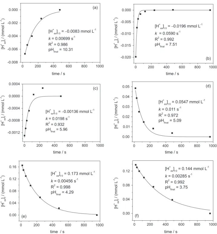
Figure 5. Evolution in time of the proton exchange ([H+
ex]t in mmol L-1) after 6 titrant additions (pHfinal from 10.31 (a) to 3.75 (f)) along the potentiometric
titration. Total exchange, [H+
ex]total, is obtained using equilibrium values (pH, Ci, βj, equation 6, of the modeling section); “slow” first-order exchange,
[H+
ex]t0, is obtained with equations 7 and 8 (of the modeling section). Note that the y-axis unity is equivalent to buffer capacity/intensity indexes, as discussed
at disturbed conditions. The first step of this kinetic model
is to derive the proton concentration difference [H+
ex](t –final)
between all the states at time “t” ([H+]
t and [OH
-]
t) of
the pH response and the “final” pseudo-equilibrium state ([H+]
final and [OH-]final), as follows:
(7)
where [OH–] = β
OH–[H+]–1
Fitting the curve [H+
ex](t–final) versus time with the following first-order rate law:
(8)
one can obtain the values for the initial “slow” proton
exchange, named [H+
ex]t0,and the first-order rate constant,
k, for each addition of titrant along the potentiometric
titration. The subscript “t0” in “[H+
ex]t0”defines a modeled
initial amount for the first-order “slow” proton exchange
at t = 0. Results of this kinetic framework, the values of
[H+
ex]t0 and k as a function of pH, are illustrated in
Figures 5, 6 and 7. In Figure 5, the values of [H+
ex]t0 are
normalized to the mass of biotite (g-1) and also to the pH
variation (∆pH-1) between related titration points n and n–1,
resulting in an exchange pattern that is a representation in terms of pH disturbance response of the given sample
(∆pH = pHfinal n-1 – pHfinal n, see Figures 1 and 2). The pH
variation, ∆pH, from one point of the titration to the
next varies from ca. 0.1 pH units in acidic conditions to ca. 1.8 pH units at pH 7-9 and 0.2 pH units at pH around 10.
“Slow” proton exchange entropy production
Kinetically-resolved potentiometric titrations can be used for the thermodynamic characterization of
out-of-equilibrium changes that drive perturbated systems toward new equilibrium, or pseudo-equilibrium state. When a studied system is perturbated (e.g., by titrant addition), it is instantly created out-of-equilibrium states that possess free energy, the proton potential difference between complex perturbated phases. If the system does not collapse, the nearest equilibrium state is reached (hence, “linear out-of-equilibrium thermodynamics” or “near equilibrium” conditions) through free-energy dissipation or entropy production. Note that in strongly or continuously perturbated systems, which are not the case in our study, “far from equilibrium” or “non-linear thermodynamics” would need to be considered. For the present biotite-water system,
the entropy production, dS/dt (in J K-1 s-1), can then be used
as an important parameter of perturbed systems to quantify the resilience of biotite to pH perturbations. The coordinate
to be considered is time.5 The “slow” kinetics as well as
the variations of pH response observed after each titration addition in the biotite-water system can be used in order to calculate the “slow” proton exchange entropy production pattern as follows. The first assumption is that perturbed states possess potential differences, generally called forces
Figure 6. First-order kinetical plot (equation 8) using data shown in Figure 2.
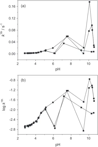
Figure 7. First-order rate constants k (s-1) in (a) and log k in (b) as a
F. The forces F drive the fluxes J. In chemical reactions,
the flux J is the reaction rate, dξ/dt, the time evolution of
reaction coordinate ξ.5 The entropy production is then
defined by the summation of the product of forces F and
fluxes J as:
dS/dt = ∑F × J (9)
Applied to chemical reactions and using the chemical
affinity A, F becomes:
F = A/T (T in Kelvin) (10)
J = reaction rate = dξ/dt (11)
Combining with equation 9, the entropy production
can be defined as:
dS/dt = ∑A(dξ/dt) / T (12)
where the chemical affinity A is
A = µreagents – µproducts (13)
In order to use these general equations (equations 9-13)
in the biotite-water system and derive and the reaction
rate (dξ/dt),we firstly defined the model as the protonation
reaction of complex system S (complex system conjugate
bases S and conjugate acids, H+S) according to the
equation:
H+ + S⇄ H+S (14)
At each point of the titration n, when pseudo-equilibrium
is reached at pHfinal n(named pHeq) a new specific modeled
equilibrium conditional constant Kn is obtained:
(15)
Since the complex system S can be modeled by the
contribution of the constituting components i (A, B, C and D) we found:
(16)
where [Si] and [H+Si] are the conjugate base and conjugate
acid concentrations of components i (A, B, C and D) with:
(17)
which defines the molar fraction xSi and xH+Siof conjugate
bases and conjugate acids of the components i. Upon
perturbation, the equilibrium condition state constant Kn
is replaced by out-of-equilibrium condition state quotient
Qn and the affinity A is defined by:
A = µreagents – µproducts = RT ln(Kn/Qn) (18)
In order to derive Qn, we used equation 14 (H+ + S⇄ H+S)
and applied the “slow” proton exchange [H+
ex]t0 as the proton concentration difference between initial condition
of the first-order proton exchange at t0 (which is a modeled
condition) and the final equilibrium condition at pHfinal
(pHeq) (see “linear out-of-equilibrium calculation” section
for derivation of [H+
ex]t0). Then is defined as:
(19)
where:
[H+S]
t0 = [H+S]eq – [H+ex]t0 (20a)
[S]t0 = [S]eq + [H+ex]t0 (20b)
and:
(21)
with
Equation 21 is the solution of the second order
polynomial, –([H+]
t0) 2 + ([H+]
t0)c + βOH–, for the substitution
of the difference [H+
ex](t− final) by the difference [H+ex]t0 in
equation 7 at t = t0. Then, we can define [H+]
t0 as the
modeled proton concentration (10–pHt0
) of the perturbed
state t0. Note that [H+]
t0 is not a difference between states
but a concentration of a unique perturbed state.
In equation 20a and equation 20b, [S]eq and [H
+S] eq, the equilibrium concentration of complex system conjugated bases and conjugate acids respectively, can be derived as follows:
(22a)
Having calculated [S]t0, [H+S]t0 and [H+]t0 in order to
derive (equation 19), and knowing Kn (equation 15), we
obtain affinity A as:
(23)
In order to solve equation 23, we should make use of
equation 22aand equation 22b and the molar fractions
of equation 17 for components i (A, B, C and D) and
related species j. In this way, we defined the perturbation
(proton exchange [H+
ex]t0) in the equilibrium model of
equation 14 (H+ + S⇄ H+S) for each titration point n, using
equilibrium parameters Ci and βj previously calculated
with Best7 software (see previous modeling sub-section and Table 1). We should remark that the approximation
of equation 23is strongly dependent on [H+]
t0, [H +]
eq and
dominant component at each pH region (e.g., component A at perturbations around pH 4).
The second term in the equation of the entropy production (equation 12) for “slow” proton exchange is
the reaction rate, dξ/dt, which is defined as:
dξ/dt = –k[H+
ex]t0 in mol L-1 s-1 (24)
Substitution of A (equation 23) and dξ/dt (equation 24)
in equation 12, results in:
(25)
with R = 8.314 J mol-1 K-1. For volume of 1 L, dS/dt is
given in J K-1 s-1.
The values calculated using equation 25 for the kinetics
of each titration point n are presented in Figure 8, normalized
by sample mass (g-1) and DpH-1 (1/(pH
final n-1− pHfinal n)).
Figure 8 is a representation of the “slow” proton entropy production of perturbed biotite-water complex systems as
a function of pH condition (pHfinal n or pHeq). Also, Table 2
presents selected symbology and description for the data treatment presented above.
The pH of the soil solution is a critical environmental parameter for the growth and health of all organisms living in the soil, i.e., bacteria, fungi and plants. Low pH in soils tend to decrease the bioavailability of macronutrients (N, P, Ca, Mg, K and S) while it increases the level of Al and Mn ions, both toxic elements for plants. As such, pH is also the main factor shaping the bacterial diversity in many natural different
soils as well as in heavily polluted soils.11,13,26 The mobility
Figure 8. Entropy production for linear out-of-equilibrium “slow” proton exchange versus pH. The representation is normalized by sample mass (g-1) and total pH variation (∆pH-1). The “slow” proton exchange
entropy production processes maximum at acid conditions represents the significant contribution of stable subsystems within the biotite which keep the water-biotite complex system resistant to acidification. The main reason for these patterns is suggested to be the heterogeneous nature of biotite-water complex system.
Table 2. Selected symbology description
Symbol Description Dimension
pHfinal n or pHeq n last measured pH of titration point “n” dimensionless
pHfinal n-1 or pHeq n-1 last measured pH of previous titration point “n–1” dimensionless
pHinitial initial “slow” kinetic measured pH dimensionless [H+]
final n proton concentration at pHfinal n, or pHeq n mol L
-1
[H+]
final n-1 proton concentration at pHfinal n-1, or pHeq n-1 mol L-1
[H+]
t proton concentration at time “t” mol L
-1
[H+]
t0 proton concentration at calculated (equations 8 and 21) initial first order kinetic condition “t0”a mol L-1
[H+]
eq proton concentration at pHfinal, or pHeq mol L-1
[H+
ex]t-final concentration difference between kinetic measured conditions at time “t” and “final”b mol L-1
[H+
ex]t0 concentration difference between calculated condition “t0” (equation 8) and “final” measured conditiona, b mol L-1
[H+
ex]total total proton exchange (equation 6)b mol L-1
of organic compounds are also strongly pH-dependent, with acidification promoting desorption reactions of organic
pesticide or herbicide (e.g., atrazine) as H+ compete for
adsorption sites at the solid surface.27 Soils tend to “resist”
to pH changes when either acid or base is added. However, measuring soil and/or mineral pH buffering capacity can be tricky as often titration methods differ in pH equilibration time after each titrant addition, varying from few minutes to
hours.25 More importantly, pH equilibration kinetics during
potentiometric titrations of soils or minerals are typically not monitored despite the fact that they can give interesting
insights into the type of reactions involving H+ at various pH
ranges, as well as, their extent and rate.
In the case of biotite, the results of the equilibrium potentiometric titration and the Best7 modeling (Figure 1, Figure 3 and Table 1) allow us to propose four different components that influence the pH buffering capacity of
biotite along the pH range studied. A prevalent component A
in acidic conditions (–log βH+Aca. 3.8) that account for 58%
of the total amount of exchanged H+ while the remaining
capacity is spread between component B (a weak acid
with –log βH+Bca. 5), component C (–logβH+Cca. 6.5)
and component D (a weak base with –logβH+Dca. 9.5).
As such biotite exhibits the characteristic phyllosilicate
structure consisting of alternating tetrahedrally T (Si4+, AlIII
or FeIII substituted and bounded to O2-) and octahedrally O
(FeII, MgII, MnII bounded to O2-) coordinated sheets (T-O-T
layers) stacked along the [001] direction with interlayer
space filled with KI. Even though this is not the scope of the
present study, we tentatively suggest that the protonation of
component Ais an average representation of protonation
reaction such as MOHx + H+⇄ MOH
2
x+1 where M could
be Si4+ (based on the surface speciation of pure quartz).28
Similarly, components B, C and D are hypothesized to be the
results of combined contribution of FeII (and/or FeIII which
account for ca. 20% of Fe total in the biotite sample),29,30
AlIII and MgII oxide/hydroxide protonation reactions.16,31
Exposure to low pH eventually lead to further protonation of three neighbouring M–O bonds which in turn will lead
to the detachment of the metal cations.32 Therefore,
proton-promoted dissolution reactions can contribute to the pH buffer capacity of the biotite-water system. Biotite cations
exchange, mainly MgII and KI only partially compensated
by protons incorporation within biotite, is also a process that
can account for H+ consumption as shown by Bray et al.18
As can be seen in Figure 1, those four calculated components and their associated equilibrium constants
provide a good fit (σfit < 0.03) to the experimental titration
curve for biotite-water system.
Combining the specific H+ mass balance equation
(equation 6) of each component i, one can obtain the total
exchangeable [H+
ex]total as a function of pH (the black
square in Figure 5). Essentially those calculations show a maximum proton exchange at pH < 5 reaching up to
8 mmol L-1 g -1∆pH-1 while, in the neutral and basic pH
ranges, the total proton exchange is limited, yet constant
between ca. 1-2 mmol L-1 g -1 ∆pH-1 (it should be noted that
since there is no experimental points at pH between 7 and 9, we should not overestimate the total proton exchange at pH 8, that should be the minimum of the black-square plot presented in Figure 5). Those values are relatively
high when compared to literature data for soils.25 It is
important to remark the influence of equilibration time between soil-water systems and titrant solutions and also the need to explore the kinetics of pH-response of mineral/ soil subjected to pH perturbations.
Using a first-order rate law for the perturbed biotite-water system, we fitted the pH response kinetics after each titrant addition as a function of pH (Figure 6). The
first-order “slow” proton exchange [H+
ex]t0 (modeling section,
equations 7 and 8) shows a similar behavior when compared
with the total exchangeable protons [H+
ex]total with a steep increase at pH < 5 (Figure 5). Yet, at neutral and basic pH
regions [H+
ex]t0 is close to 0 or even negative at pH > 10.
The difference between total proton exchange [H+
ex]total and
“slow” proton exchange [H+
ex]t0 is due to the fact that [H+ex]t0 is determined from the “slow” pH response alone (first-order equilibration decay from maximum of 30 s to 960 s
after titrant addition) while total [H+
ex]total exchangeable proton is derived from the whole equilibrium titration curve (see modeling section, equation 6). We interpret this “slow”
proton exchange [H+
ex]t0 minimum value to reflect the low
reactivity of the biotite in term of dissolution at pH > 5 as
reported by Bonneville et al.23 The low amount of [H+
ex]t0 at neutral and basic pH confirms also that the release of
interlayer cations, i.e., KI which is independent of pH, is
only partially compensated by the H+ incorporation as
already shown in Bray et al.18 Hence, it is likely that, in
neutral/basic pH range, biotite develops a negative charge.
With respect to rate constant k, we observe the lowest values
in the acidic range which is in consistency with processes of “slow” kinetics such as dissolution reactions (we should remark that diffusion phenomena may contribute in the whole observed out-of-equilibrium “slow” proton exchange, but the whole phenomena was simplified, for convenience, as an entire first-order chemical reaction). The
k values tend to increase as pH become neutral and basic
(Figure 7), this trends might suggest different fast proton
exchange processes such as KI or MgII substitution, fast
protonation of vertex, edges, and crystal defects.
observations to reveal the “slow” proton exchange entropy production of the biotite-water system in relation to titrant perturbation (in this case with 0.1 mL aliquot additions
of 0.1019 mol L-1 HCl). Generally, out-of-equlibrium
states can be defined by their stability as a function of time. Stable systems maintain slow out-of-equilibrium processes while unstable systems, upon perturbations, evolve quickly to a new pseudo-equilibrium state. Since change is driven by difference (negentropy or energy input) we use entropy production as a fundamental description of
systems stability as discussed below.5 As mentioned, it is
important here to distinguish “fast” from “slow” out-of-equilibrium processes. Due to experimental limitations, the “fast” out-of-equilibrium processes (occurring in less than 30 s after perturbation) cannot be precisely measured.
However, by the difference between the total ([H+
ex]total)
and the “slow” ([H+
ex]t0) proton exchange as defined in
equation 6 and equation 8, respectively, it is possible to estimate the magnitude of the “fast” proton exchange. The contribution of the “fast” out-of-equilibrium processes is particularly significant in the neutral/basic pH range (where “slow” proton exchange is close to zero). We can propose that the “fast” contributions are probably related to
modeled components B, C and D.As observed in Figure 6,
above pH 4.5, those “fast” out-of-equilibrium processes contributes for most of the total proton exchange and this is achieved in a very short time period (less than 30 s) of the pH-response to perturbation, which is indicative of a high entropy production (“fast” contribution exchange rate is always bigger than the rate of remaining “slow” proton exchange, as can be logically proposed). These “fast” proton exchanges (at neutral/basic pH conditions) can be related to the exchange contribution of the biotite complex subsystems that rapidly evolve to a new pseudo-equilibrium state, a characteristic behavior of relatively unstable subsystems which are less resistant to titrant perturbations. In contrast, when “slow” processes occur, we can interpret
it as a priori stable subsystems processes as defined by the
minimum entropy production principle.5 In this context, the
derivation of “slow” proton exchange entropy production is a quantification of the performance of stable constituents of the biotite during the potentiometric titration. We showed
in modeling section that by using Ci, βj, [H+ex]t0 and k, it
is possible to calculate the entropy production dS/dt of
the “slow” proton exchange processes, as a function of
the pH condition, sample mass (g-1) and pH disturbance
(∆pH-1). When “slow” rate proton exchange occurs as a
result of potentiometric titration perturbations, one can define simple assumptions that relate the measured data
with fundamental thermodynamic concepts, the forces F
and fluxes J. Generally the forces F can be represented by
the affinity A (see modeling section). In the irreversible
“slow” proton exchange the processes are governed by
the amount of exchangeable proton [H+
ex] and when the
pseudo-equilibrium is reached the net exchange tends to
zero, so the forces and so the affinity .
Figure 8 is the representation of the “slow” proton exchange entropy production. It suggests that biotite offer a significant stable pressure against acidification of water in natural settings. The perturbations of the biotite-water system to acid pH states are slowly counter-balanced by large proton consumption, dissipating the energy (producing entropy) introduced by the titrant additions. In other words, at acidic conditions the “slow” proton exchange is large and can be maintained for long time
periods (at least 960 s with k lower than 0.01 s-1). In contrast,
at basic/neutral pH conditions we observed only “fast” proton exchange that, even being significant in quantitative terms (almost 40% of total buffering capacity, see Figures 4, Figure 5 and Table 1), occurs in short time periods (less than 30 s). As mentioned, the peak of “slow” proton exchange entropy production of biotite in acidic conditions (Figure 8) is heavily influenced by the large proton amount that is
exchangeable [H+
ex]t0, even though first-order rate constants
are small (note also the small total pH variations between pHfinal n-1 and pHfinal n at acidic pH conditions in Figure 1).
It is also interesting to emphasize the difference of the biotite-water system with other chemical systems and other soil constituents. For instance, for soluble low-molecular weight organic acids such as phtalic acid, the titrations and the proton exchanges are generally dominated by fast processes. On the other hand, depending on the system exposed to perturbations, the pH-responses can be slower and restricted to specific pH regions, similarly as observed in the biotite-water system at acidic pH conditions. In
the case of saprophitic fungi Trametes villosa it is quite
different, perturbated states present a large extent of
“slow” proton exchange at basic pH conditions.20 In
yet unpublished work, we have found that humic acids present significant “slow” proton exchange processes at neutral/basic pH conditions (between pH 6.5 and 9). It can be hypothesized that the relation between water and minerals such as biotite contribute to avoid acidification, while bacteria, organic matter and fungi contribute to avoid extensive basification since that organic matter and biological systems, such as humic substances and microorganisms, show semi-complementary features with “slow” proton exchange reactions at neutral/basic
pH conditions.20 Indeed, other behavior can be observed
circadian effects (most in the case of living organisms), experimental batch size, type and amount of perturbant, year seasons of sample collection (most for forest soils),
symbiosis effects, and other.13,17,20,26,33 In general, healthy
soil components play as proton pressure elements that maintain the water environment near neutrality, providing chemical conditions to soil processes to occur without high energy costs. The balance of proton exchange amount and respective rates constants may indicate the evolution of the given model systems. Also, it could mean that upon disturbance, the soil components (microorganisms, organic matter and soil aggregates) that intimately interact with biotite will undergo slower or mitigated microenvironment pH variations and acidification. In the case of biotite, the evolution towards basic pH conditions seems to occur easily and over short timescale but acidification will demand high proton input and long time in the evolution period. During alteration experiments in the micro-environment of living mycorrhiza (symbiotic association between fungi and
tree-roots) Bonneville et al.23 showed that the biotite surface
micro-environment can be strongly perturbed probably due to living fungi acidic exudates and/or weathering with the pH condition stabilizing around pH 4 after a significant pH decrease from pH 6.5, which is in good agreement with the present results on biotite pH perturbation stability properties. It is important to emphasize the necessary precaution in the interpretation of the ontological differences between controlled experiments and soil processes occurring in the environment (the most important problem, among several, is that natural conditions are usually “far from equilibrium” and it is not trivial, or even possible, to point linear relations between laboratory measurements and ecological processes). Nevertheless, as mentioned earlier, soil is a complex organization for which there is, so far, few information concerning their time pH-responses facing perturbations. For instance, even though some species of fungi and some organic matter compounds have been investigated, further research is needed in order to address the pH response of bacteria for instance, an important living soil component. However, the methodology developed here can be easily applied to simple constituent of soils or eventually to raw soil samples. Established the necessary epistemological precautions and the interesting complexity of the soils subject, we propose that the development of models, such as presented here, offer transversal points of view for complex system studies based on difference and heterogeneity in ecology and biogeochemistry. The construction of perturbation response patterns could also be useful for field research in agroecology and in the study of relations between phenomenological change observation and the cosmovision of researchers, students, and all other
soil “users” and their different development of signification,
as suggested in a transdisciplinary field.2-5,8,10
Conclusions
We proposed that the simple method shown herein is a powerful tool for potentiometric (pH) complex systems studies, mainly soil components and/or raw soils. Also, it is important to remark that the results are products of a hybrid model on equilibrium and linear out-of-equilibrium measurements using the glass-electrode as an accessible intermediate technology. Beyond the physicochemical applicability of this methodology for earth sciences (with the obtainment of proton flux, rate constants and entropy production as parameters for the construction of complex systems change patterns and stability), it is proposed that this work plays as a pedagogical tool for model development in transdisciplinary landscape complexity studies.
Acknowledgments
We thank CNPq (The Brazilian National Council for Technological and Scientific Development), the Federal University of Santa Catarina (UFSC) and the Université Libre de Bruxelles (ULB) for financial support and Lei Chou and Nathalie Roevros for technical help in the laboratory. Steeve Bonneville benefits from the support of the fund “Victor Brien” and from the fund “Van Buuren”.
References
1. Naveh, Z.; Landscape Urban Plan.2007, 57,269.
2. Morin, E.; Ciência com Consciência, 14th ed.; Bertrand Brasil:
Rio de Janeiro, 2010.
3. Bateson, G.; Steps to an Ecology of Mind; J. Aranson: Northvale, 1987.
4. Maturana, H.; A Ontologia da Realidade; Humanitas: Belo Horizonte, 1997.
5. Kondepudi, D.; Prigogine, I.; Modern Thermodynamics; Wiley: Chichester, 1998.
6. Martell, A. E.; Motekaitis, R. J.; Determination and Use of Stability Constants; VHC Publishers: Dallas, 1992.
7. Motekaitis, R. J.; Martell, A. E.; Can. J. Chem.1982, 60, 2403. 8. Primavesi, A.; Manejo Ecológico do Solo, 7th ed.; Nobel: São
Paulo, 1984.
9. Ponizovskiy, A. A.; Pampura, T. V.; Eurasian Soil Sci.1993, 25, 79.
10. Altieri, M.; Agroecologia, 2nd ed.; FASE: Rio de Janeiro, 1989.
12. Stumm, W.; Morgan J. J.; Aquatic Chemistry; Wiley: New York, 1995.
13. Stumm, W.; Chemistry of the Solid-Water Interface; Wiley: New York, 1992.
14. Nesbitt, H. W.; Young, G. M.; Geochim. Cosmochim. Acta1984, 48, 1523.
15. Sposito, G.; The Surface Chemistry of Soils; Oxford University Press: Oxford, 1984.
16. Baes, C. F.; Mesmer, R. E.; The Hydrolysis of Cations; Wiley: Michigan, 1976.
17. Kazakov, S.; Bonvouloir, E.; Gazaryan, I.; J. Phys. Chem. B
2008, 112, 2233.
18. Bray, A. W.; Benning, L.; Bonneville, S.; Oelkers, E. H.; Geochim. Cosmochim. Acta 2014, 128, 58.
19. Baidoo, E.; Ephraim, J. H.; Darko, G.; Geoderma2014, 217, 18.
20. Almeida, V. R.; Szpoganicz, B.; Open J. Phys. Chem. 2013, 3, 189.
21. Escandar, G. M.; Sala, L. F.; J. Chem. Edu.1997, 74, 1329. 22. Rifkin, J.; Howard, T.; Entropy;Viking Press: New York, 1980. 23. Bonneville, S.; Morgan, D. J.; Schmalenberger, A.; Bray,
A.; Brown, A.; Banwart, S. A.; Benning, L. G.; Geochim. Cosmochim. Acta2011, 75, 6988.
24. Souza, M. M. S.; Arend, K.; Fernandes, A. N.; Giovanela, M.; Szpoganicz, B.; Anal. Chim. Acta2001, 445, 89.
25. Ivanova, S. E.; Solokova, T. A.; Moscow Univ. Soil Sci. Bull.
1998, 53, 12.
26. Valentin-Vargas, A.; Root, R. A.; Neilson, J. W.; Chorover, J.; Maier, R. M.; Sci. Total Environ. 2010, 500, 314.
27. Brady, C. N.; Weil, R.; Elements of Nature and Properties of Soils, 3rd ed.; Pearson Education International: London, 2010.
28. Duval, Y.; Mielczarski, J. A.; Pokrovsky, O. S.; Mielczarski, E.; Ehrhardt, J. J.; J. Phys. Chem. B2002, 106, 2937.
29. Liger, E.; Charlet, L.; van Cappellen, P.; Geochim. Cosmochim. Acta1999, 63, 2939.
30. Rosenqvist, J.; Persson, P.; Sjoberg, S.; Langmuir2002, 18, 4598.
31. Pokrovsky, O. S.; Schott, J.; Geochim. Cosmochim. Acta2004, 68, 31.
32. Schwertmann, U.; Plant and Soil1991, 130, 1.
33. Gow, N. A. R.; Robson, G. D.; Gadd, G. M.; The Fungal Colony; C.U. Press: New York, 1999.
Submitted: March 20, 2015