UNIVERSIDADE DE ÉVORA
DEPARTAMENTO DE ECONOMIA
DOCUMENTO DE TRABALHO Nº 2005/10
June
Bootstrap bias-adjusted GMM estimators
Joaquim J. S. Ramalho*Universidade de Évora, Departamento de Economia, CEMAPRE
* The author gratefully acknowledges partial financial support from Fundação para a Ciência e Tecnologia, program POCTI,
partially funded by FEDER. Address for correspondence: Joaquim J. S. Ramalho, Universidade de Évora, Departmento de Economia, 7000-803 ÉVORA, Portugal. Tel.: +351-266740894. Fax: +351-266740809.
E-mail: [email protected].
UNIVERSIDADE DE ÉVORA
DEPARTAMENTO DE ECONOMIA
Largo dos Colegiais, 2 – 7000-803 Évora – Portugal Tel.: +351 266 740 894 Fax: +351 266 742 494
Abstract:
The ability of six alternative bootstrap methods to reduce the bias of GMM parameter estimates is examined in an instrumental variable framework using Monte Carlo analysis.
Promising results were found for the two bootstrap estimators suggested in the paper.
Palavras-chave/Keywords: GMM, Bootstrap, Empirical Likelihood, Instrumental Variables, Monte Carlo
1
Introduction
It is now widely recognized that the efficient two-step generalized method of moments (GMM) es-timator may have large biases for the sample sizes typically encountered in economic applications; see, for example, the several Monte Carlo studies that appeared in the July 1996 special issue of the Journal of Business & Economic Statistics. In this paper we analyze the ability of six alter-native bootstrap procedures to reduce the finite sample bias of GMM parameter estimates. Three of those alternatives were already proposed by other authors: the standard, nonparametric (NP) bootstrap; Hall and Horowitz’s (1996) recentered nonparametric (RNP) bootstrap; and Brown and Newey’s (2002) constrained empirical likelihood (CEL) bootstrap. Monte Carlo evidence by Horowitz (1998) and Ramalho (2005) shows that application of these bootstrap methods reduces the bias of the GMM estimator but does not completely eliminate it. Therefore, in this paper we suggest two alternative bootstrap techniques, both of which use the empirical likelihood (EL) distribution function (see Qin and Lawless, 1994) to generate the bootstrap samples. The finite sample bias of all the corresponding bootstrap bias-corrected GMM estimators are examined in an instrumental variable framework through a Monte Carlo analysis.
2
GMM estimation
Let yi, i = 1, ..., n, be independent and identically distributed observations on a data vector y, θ
a k-dimensional vector of parameters of interest, and g (y, θ) an s-dimensional vector of functions of the observed variables and parameters of interest. Throughout, we assume that s > k and that
the true parameter vector θ0 uniquely satisfies the moment conditions
EF[g (y, θ0)] = 0, (1)
where EF[·] denotes expectation taken with respect to the unknown distribution function F (y).
Define gi(θ) ≡ g (yi, θ), i = 1, ..., n, and gn(θ) ≡ n−1
Pn
i=1gi(θ). Regularity conditions are
assumed such that gn(θ)
p
→ EF [g (y, θ)]and√ngn(θ0)
d
→ N (0, V ), where the asymptotic variance
matrix V ≡ EF
£
gi(θ0) gi(θ0)0
¤
is positive definite and→ andp → denote convergence in probabilityd
and convergence in distribution, respectively.
The efficient GMM estimator ˆθGMM is obtained from minimization of the optimal quadratic
form of the sample moment indicators
Qn= gn(θ)0 h Vn ³ ˜ θ´i−1gn(θ), (2)
where ˜θ is a preliminary consistent estimator for θ0 and ˜Vn ≡ Vn ³ ˜ θ´ is a consistent estimator for V . Let G ≡ EF h∂g i(θ0) ∂θ0 i
. Under suitable regularity conditions, see Newey and
McFad-den (1994), ˆθGM M is a consistent, asymptotically normal estimator of θ0, √n
³ ˆ
θGMM− θ0
´ d
→
Nh0, (G0V−1G)−1i, and is asymptotically efficient among all estimators based only on (1).
3
The empirical likelihood distribution function
Consider again the moment conditions (1). Implicitly, by giving the same weight (n−1) to each
observation, GMM uses the empirical distribution function Fn(y)≡ n−1
Pn
i=11 (yi ≤ y) as
esti-mate for F (y), where the indicator function 1 (yi ≤ y) is equal to 1 if yi ≤ y and 0 otherwise.
However, since the moment conditions (1) are assumed to be satisfied in the population, this information can be exploited in order to obtain a more efficient estimator of F (y). Actually, we
may obtain an alternative estimator for θ in (1) by choosing the estimator ˆθ that minimizes the
distance, relatively to some metric, between Fn(y) and a distribution function Fp(y) satisfying
the moment conditions (1). The distribution Fp(y) is, hence, the member of the class F (θ) of all
distribution functions that satisfy (1), F (θ) ≡©Fp : EFp[g (y, θ0)] = 0
ª
, that is closest to Fn.
In the selection of a particular probability measure in F (θ), different metrics for the closeness
between Fp(y)and Fn(y)may be used. The most common choices for the metric M (Fn, Fp)are
particular cases of the Cressie-Read (1984) power-divergence statistic, namely M (·) =PdFn(y)
ln [dF n (y) /dFp(y)] which produces the so-called EL estimator. Thus, the EL estimator ˆθELcan
be described as the solution to the program max θ n X i=1 ln pELi subject to pELi ≥ 0, n X i=1 pELi = 1 and n X i=1 pELi g (yi, θ) = 0, (3)
where pELi ≡ dFp(yi), i = 1, ..., n, and the last restriction is an empirical measure counterpart to
the moment conditions (1), imposing them numerically in the sample; for an alternative motiva-tion of EL estimators, see Newey and Smith (2004).
From optimization of (3), it is straightforward to show that ˆ pELi ≡ p EL i ³ ˆ θEL, ˆλEL ´ = 1 nh1 + ˆλ0ELg³yi, ˆθEL ´i, i = 1, ..., n, (4)
where ˆθEL and ˆλEL, the s-vector of Lagrange multipliers associated to the last restriction of (3),
result from unconstrained optimization of the saddle function n−1Pn
i=1ln [1 + λ0gi(θ)]. Thus,
the EL distribution function Fp(y) is given by Fp(y) = n X i=1 ˆ pELi 1 (yi ≤ y) . (5)
See Qin and Lawless (1994) for details.
4
Alternative bootstrapping for the GMM estimator
Assume that a random sample S of size n is collected from a population whose (unknown) distribution function is F (y). Bootstrap samples are generated by randomly sampling S with
replacement. This resampling is based on a certain distribution function, F∗(y), which assigns
each observation a given probability of being sampled. In general, using the bootstrap, the bias
of the GMM estimator ˆθGM M can be estimated as follows: 1) compute ˆθGM M by minimizing
(2) based on S; 2) generate B bootstrap samples Sj∗, j = 1, ..., B, of size n accordingly with
the chosen F∗(y): S∗
j = © y∗ j1, ..., y∗jn ª , where y∗
ji, i = 1, ..., n, denotes the observations included
in the bootstrap sample S∗
j; 3) for each bootstrap sample calculate the GMM estimator ˆθ
∗ j ≡ arg min θ g ∗ jn(θ) ˆVjn∗−1gjn∗ (θ), j = 1, ..., B, where gjn∗ (θ) = n−1 Pn i=1g ¡ y∗ ji, θ ¢
and ˆVjn∗−1 uses a
pre-liminary consistent estimator for θ0 based on the bootstrap sample Sj∗; 4) average the B GMM
estimators calculated in the preceding step: ¯θ∗ = B1 PBj=1ˆθ∗j; 5) estimate the bias of the GMM
estimator ˆθ by calculating:
ˆb = ¯θ∗
− ˆθGM M. (6)
Subtracting the bias (6) from the GMM estimator ˆθGM M, it is then possible to obtain the
bias-corrected GMM estimator
ˆ
θBCGMM = 2ˆθGMM− ¯θ∗. (7)
As discussed next, these general procedures may be used to reduce the finite sample bias of GMM parameter estimates in several distinct forms.
4.1
Nonparametric bootstrap
The NP bootstrap is probably the most commonly applied bootstrap technique in econometrics.
In this case, the bootstrap samples are generated using the empirical distribution function Fn(y),
so each observation has equal probability n−1 of being drawn. However, direct application of
the NP bootstrap in the GMM framework seems to be unsatisfactory in many cases. Indeed,
satisfied at θ = θ0, the estimated sample moments are typically non-zero, that is, there is no θ
such that EFn[g (y, θ)] = 0 is met, except in very special cases. Therefore, Fn(y) may be a poor
approximation to the true underlying distribution of the data and, hence, the NP bootstrap may not yield a substantial improvement over first-order asymptotic theory in standard applications of GMM.
4.2
Recentered nonparametric bootstrap
In order to guarantee that the moment conditions exploited by GMM estimators hold exactly in each replication of the bootstrap, Hall and Horowitz (1996) suggested using the recentered moment indicators gc¡yj∗, θ ¢ = g¡yj∗, θ ¢ −n1 n X i=1 g³yi, ˆθGM M ´ , (8) since EFn £ gc¡yj∗, θ ¢¤
= 0. To implement this RNP bootstrap method some adaptations must be made to the general procedures described earlier. Namely, in step 1 we have to calculate also gn
³ ˆ
θGM M
´
and in step 3 GMM estimation is now based on the recentered moment indicators (8), with the weight matrix specified accordingly.
4.3
Constrained empirical likelihood bootstrap
Instead of recentering the moment conditions and keeping Fn(y) as resampling distribution,
Brown and Newey (2002) suggested generating the bootstrap samples using a different
distribu-tion, say F1(y), such that EF1
h
g³y, ˆθGM M
´i
= 0. Namely, they proposed the employment of a constrained version of the EL distribution function (5), which is given by
Fpc(y) = n X i=1 ˆ pCELi 1 (yi ≤ y) , (9) where ˆ pCELi = 1 nh1 + ˆλ0CELg ³ yi, ˆθGM M ´i, i = 1, ..., n, (10)
and ˆλCEL results from maximization of n−1
Pn i=1ln h 1 + λ0gi ³ ˆ θGMM ´i ; in other words, Fc p (y)
results from solving the program (3) conditional on θ = ˆθGM M. Since Pni=1pˆCELi gi
³ ˆ
θGM M
´ =
0 is the first-order condition characterizing ˆλCEL, this CEL bootstrap imposes, in effect, the
moment conditions, evaluated at ˆθGM M, on the sample: EFCEL
h
g³y, ˆθGMM
´i = 0.
Brown and Newey (2002) proved that the CEL bootstrap is asymptotically efficient relative
to the NP and RNP methods, since Fc
p(y) is a more efficient estimator of F (y) than Fn(y).
4.4
Recentered empirical likelihood bootstrap
The two bootstrap methods that we propose in this paper are based on the EL distribution
Fp(y)given in (5). Although they are not expected to be more efficient than the CEL bootstrap,
the fact that Fp(y) is used instead of Fpc(y) may lead to better results in finite samples for two
reasons: first, the former distribution do not result from an optimization conditional on θ = ˆ
θGM M as the latter; second, there are some Monte Carlo evidence suggesting that ˆθEL displays
less bias than ˆθGM M in small samples; see inter alia Ramalho (2005).
As before, some correction seems to be necessary to apply this EL bootstrap to the GMM
estimator, sincePni=1pˆEL
i g
³
yi, ˆθGM M
´
6= 0 in general. Analogously to Hall and Horowitz (1996), we suggest using the recentered moment indicators
gc¡y∗j, θ¢= g¡y∗j, θ¢− n X i=1 ˆ pELi g³yi, ˆθGM M ´ , (11) since EFEL £ gc¡y∗ j, θ ¢¤
= 0. This recentered EL (REL) bootstrap can be implemented applying similar procedures to those described for the RNP method, with only two (obvious) alterations:
Fp(y)is used instead of Fn(y) and (11) instead of (8).
4.5
Post-hoc empirical likelihood bootstrap
The expected failure of the EL bootstrap in providing significantly less biased GMM estimators can be also explained as follows. Let pEL=¡pˆEL1 , ..., ˆpELn
¢
be the n-dimensional resampling vector that assigns each observation a given probability of being sampled in the EL bootstrap. By using this resampling vector and estimating the bias utilizing the formula given in (6), we are not adequately estimating the bias of the GMM estimator that we intended to correct. Actually, in the calculation of (6), we are comparing GMM estimators that can be based on quite distinct
samples: while ˆθGM M results from the minimization of the quadratic form (2), ¯θ∗ is the average
of the standard GMM estimators ˆθj, j = 1, ..., B, each of which, due to the way the bootstrap
samples are constructed, can be interpreted as minimizing also (2) but with gn(θ) replaced by
gp(θ) ≡
Pn
i=1pˆ EL
i g (yi, θ), which, in small samples, can be rather different. Based on these
arguments, we suggest below the post-hoc EL (PHEL) bootstrap, which uses a post-sampling
adjustment to the EL bootstrap GMM estimator.1
Define pa j ≡ ¡ pa j1, ..., pajn ¢
as the actual or post-resampling vector calculated from the bootstrap
sample Sj∗, that is paji = #
©
yji∗ = yi
ª±
n is the proportion of times that the i-th original data
point appeared in the bootstrap sample S∗
j. Define also the average post-resampling vector ¯pa ≡
(¯pa
1, ..., ¯pan) = B−1
PB
j=1paj. In this framework, the j-th bootstrap estimator ¯θ
∗
j can be expressed
as a function of the j-th post-resampling vector: ¯θ∗j = θ¡pa
j
¢
. Similarly, we have for the original
GMM estimator ˆθGM M = θ (p0), where p0 = (n−1, ..., n−1). Define also ˆθ
a
= θ (¯pa) as the GMM
estimator resultant from the application of the average post-sampling probabilities ¯pa, i.e. based
on ¯ga(θ) =Pn
i=1p¯aig (yi, θ).
Instead of using ˆb = ¯θ∗− θ (p0), we propose the calculation of the bias of the GMM estimator
as:
¯b = ¯θ∗
− θ (¯pa). (12)
The intuition behind this is the following. Although the theoretical expectation of the resampling
vector pEL is p0, its actual average is ¯pa. Thus, using θ (¯pa) instead of θ (p0) in the estimation
of the bias, we might be able to correct for this discrepancy. In fact, in (12), we are effectively comparing GMM estimators based on similar samples, in opposition to what was happening before. The bias-corrected GMM estimator is then found by calculating:
ˆ
θBCGM M = ˆθGM M − ¯θ∗ + ˆθ
a
. (13)
When both n and B go to infinity, ˆθa will converge to ˆθGM M, so asymptotically this method will
produce the same results as the other bootstrap techniques discussed in the previous sections.
Note that we could have also opted for estimating the bias by ¯b = ¯θ∗ − θ¡pˆEL¢, since ¯pa ' ˆpEL.
However, the utilization of the post-resampling probabilities are expected to provide a slight further improvement.
In terms of procedures, the algorithm presented earlier must be modified as follows. In step
3, for each bootstrap sample, in addition to the GMM estimator ¯θ∗j, we calculate also paj. In step
4, the average post-resampling vector ¯pa needs also to be calculated. In the final step, we need
to obtain ˆθa and, instead of (6), the bias is calculated according to (12).
5
Monte Carlo simulation
Consider the linear instrumental variable model described by equations Yi = θ0 · Xi+ i, Xi = s X j=1 π· Zij+ ui, 7
where Yi and Xi denote the dependent variable and an exogenous regressor, respectively. All
the instruments Zij are i.i.d. N (0, Is) variables, while ( i, ui)0 is N (0, Ω), where Ω is a (2 ×
2)-matrix with diagonal and off diagonal elements 1 and ρ, respectively. We considered three different
degrees of non-orthogonality between Xiand i, ρ = (0.25, 0.50, 0.75). Let R2f = sπ2/ (sπ2+ 1)be
the theoretical R2 of the first stage regression, which measures the overall fit of the instruments
to the endogenous regressor Xi. We fix s = 10 and set the value of π in such a way that
R2
f = (0.15, 0.30) in all the experiments. The value of θ0 was fixed in order to keep constant the
overall fit of Yi to Xi in the structural equation (R2 = 0.5). For each one of the 6 parameter
combinations of s, Rf2, and ρ we generated 5000 Monte Carlo samples of size n = 200.
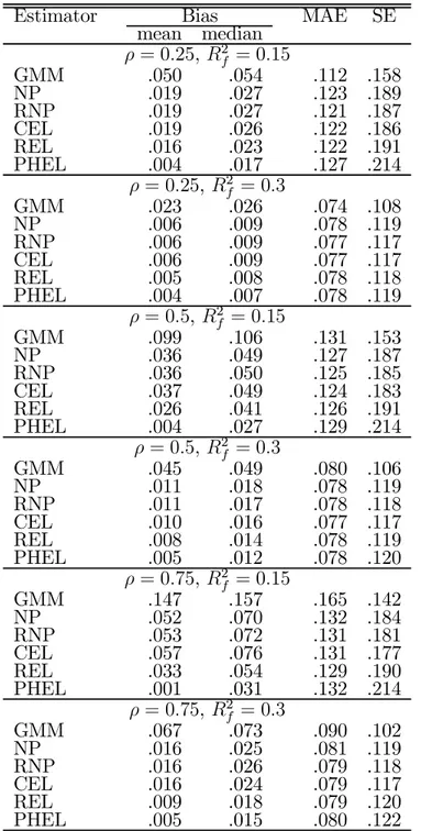
In Table 1 we report for each estimator the mean and median bias, the median absolute error (MAE), and the standard error (SE) across replications. As expected, the bias of the GMM estimator increases with the endogeneity of the model and decreases with the strength of the instruments. The same pattern can be observed for all the bootstrap GMM estimators. The utilization of any one of the bootstrap methods allows the bias of the GMM estimator to be substantially reduced, although at the expense of an increment in its dispersion. Clearly, the two estimators suggested in this paper display the best performances in terms of mean and median bias, particularly the PHEL bootstrap, which produces the only estimator which is approximately mean unbiased in all cases. Conversely, the Monte Carlo distribution of this estimator is slightly more disperse. Overall, these results suggest that the estimators developed in this paper will be useful, at least, in settings similar to those replicated in this Monte Carlo study.
References
Cressie, N. and T.R.C. Read, 1984, Multinomial goodness-of-fit tests, Journal of the Royal Statistical Society Series B 46(3), 440-464.
Brown, B.W. and W.K. Newey, 2002, Generalised Method of Moments, Efficient Bootstrapping, and Improved Inference, Journal of Business and Economic Statistics 20, 507-517.
Efron, B., 1990, More efficient bootstrap computations, Journal of the American Statistical Association 85(409), 79-89.
Hall, P. and J.L. Horowitz, 1996, Bootstrap critical values for tests based on generalised-method-of-moments estimators, Econometrica 64(4), 891-916.
Horowitz, J.L., 1998, Bootstrap methods for covariance structures, Journal of Human Resources 33(1), 39-61.
Newey, W.K. and D. McFadden, 1994, Large sample estimation and hypothesis testing, in: R.F. Engle and D.L. McFadden, eds., Handbook of Econometrics, Vol. 4 (North-Holland, Amsterdam) 2111-2245.
Newey, W.K. and R.J. Smith, 2004, Higher order properties of GMM and generalized empirical likelihood estimators, Econometrica 72(1), 219-255.
Qin, J. and J. Lawless, 1994, Empirical likelihood and general estimating equations, Annals of Statistics 22(1), 300-325.
Ramalho, J.J.S., 2005, Small sample bias of alternative estimation methods for moment condition models: Monte Carlo evidence for covariance structures, Studies in Nonlinear Dynamics and Econometrics, forthcoming.
Table 1: Monte Carlo results (5000 replications; n = 200; s = 10)
Estimator Bias MAE SE
mean median ρ = 0.25, R2 f = 0.15 GMM .050 .054 .112 .158 NP .019 .027 .123 .189 RNP .019 .027 .121 .187 CEL .019 .026 .122 .186 REL .016 .023 .122 .191 PHEL .004 .017 .127 .214 ρ = 0.25, R2f = 0.3 GMM .023 .026 .074 .108 NP .006 .009 .078 .119 RNP .006 .009 .077 .117 CEL .006 .009 .077 .117 REL .005 .008 .078 .118 PHEL .004 .007 .078 .119 ρ = 0.5, R2 f = 0.15 GMM .099 .106 .131 .153 NP .036 .049 .127 .187 RNP .036 .050 .125 .185 CEL .037 .049 .124 .183 REL .026 .041 .126 .191 PHEL .004 .027 .129 .214 ρ = 0.5, R2 f = 0.3 GMM .045 .049 .080 .106 NP .011 .018 .078 .119 RNP .011 .017 .078 .118 CEL .010 .016 .077 .117 REL .008 .014 .078 .119 PHEL .005 .012 .078 .120 ρ = 0.75, R2f = 0.15 GMM .147 .157 .165 .142 NP .052 .070 .132 .184 RNP .053 .072 .131 .181 CEL .057 .076 .131 .177 REL .033 .054 .129 .190 PHEL .001 .031 .132 .214 ρ = 0.75, R2 f = 0.3 GMM .067 .073 .090 .102 NP .016 .025 .081 .119 RNP .016 .026 .079 .118 CEL .016 .024 .079 .117 REL .009 .018 .079 .120 PHEL .005 .015 .080 .122