Brazilian Journal of Physics, vol. 34, no. 4B, December, 2004 1651
Small Scale Magnetic Field Evolution In The First
Objects Formed In The Universe
Alejandra Kandus, Reuven Opher,
Departamento de Astronom´ıa, IAG-USP, Rua do Mat˜ao 1226, Cidade Universit´aria, CEP: 05508-900, S˜ao Paulo, SP, Brazil
and Saulo M. R. Barros
Departamento de Matem´atica Aplicada, IME-USP, Rua do Mat˜ao 1010, Cidade Universit´aria, CEP: 05508-900, S˜ao Paulo, SP, Brazil
Received on 2 February, 2004; revised version on 19 May, 2004
Large scale magnetic fields in galaxies are thought to be generated, by a mean field dynamo. In order to have generated the fields observed, the dynamo would have had to have operated for a sufficiently long period of time. However, magnetic fields of similar intensities to the one in our galaxy, are observed in high redshift galaxies, where a mean field dynamo would not have had time to produce the observed fields. MHD turbulence produces small scale magnetic fields at a faster rate than it does mean fields, which can diffuse toward larger scales. If the turbulence is helical, magnetic fields generated at small scales can become correlated over large scales. We study the evolution of magnetic field correlations in the first objects formed in the universe, due to the action of a turbulent, helical, stochastic dynamo, for redshifts5≤z≤10. Ambipolar diffusion can play a significant role in this process due to the low level of ionization of the gas in the first objects. We show that for reasonable values of the parameters that characterize the turbulent plasma in the time interval considered, fields can grow to high intensities (∼µG), with large coherence lengths (∼2−6kpc).
1
Introduction
The physical processes proposed to explain the origin and evolution of the magnetic fields detected in galaxies and clusters of galaxies, can be divided into two main classes: 1) cosmological mechanisms and 2) local astrophysical pro-cesses [1, 2]. Until now, neither of them has provided a satisfactory explanation for the generation of the magnetic fields observed.
In order to explain the fields observed in our galaxy and in small redshift galaxies, a mean field dynamo is commonly invoked [3]. The dynamo would have had to have operated for a time on the order of the age of the universe to have attained the observed intensities. However, the presence of equally intense and coherent fields in high redshift galaxies [4, 5], where the mean field dynamo would not have had enough time to amplify the field to the observed values, casts doubt on the mean field dynamo paradigm as the preferred generation mechanism.
The incidence of star formation regions of the highest in-tensity increases monotonically with redshift [6]. Therefore the rate of occurrence of supernovae was also higher in the past than at present. Supernovae shocks disturb the plasma in which they are immersed, producing turbulent motions of the gas. If the occurence of supernovae was much higher in the past than at the present, the plasma of the first formed objects must have been more turbulent than observed galac-tic plasmas at low redshifts.These first stars that formed in the universe began to reionize the gas. Therefore the tur-bulence is MHD turtur-bulence, with a degree of ionization far
from complete or homogeneous.
It is known that MHD turbulence generates stochastic magnetic fields (magnetic noise) at a faster rate than mean fields. If the turbulence is strongly non-helical, the fields in-duced are confined to small scales [7, 8]. However if it is helical, magnetic field correlations over large scales occurs [9, 8].
In this study, we explore the hypothesis that the mag-netic fields observed in high redshift galaxies are created by small scale, stochastic, turbulent helical dynamos, rather than mean field dynamos. Following Ref. [8], we take into account the backreaction of the growing magnetic fields on the turbulent plasma, in the form of ambipolar diffusion. The corresponding equations for the stochastic dynamo are therefore nonlinear in the magnetic field, producing a scale of coherence larger than those in linear theory.
2
Our Model
We study a gas cloud that is assumed to have collapsed at a high redshift,z > 10. Atz ∼10, the cloud would have had a low magnetization level and a high level of turbulence. Thus, it would have been similar to the turbulent, low ioni-zation molecular clouds observed in our galaxy, albeit with a much smaller initial magnetic field and a higher level of turbulence.
1652 Alejandra Kanduset al.
redshift galaxies, modifying the plasma turbulence as they do in our galaxy. We take into account phenomenologically, the effect of cosmic rays, supernova shocks, and powerful stellar winds from massive stars by varying the turbulent pa-rameters over a broad range.
2.1
Magnetic field evolution equations
The evolution equation for the magnetic field is given by the induction equation
∂B/∂t=∇ ×(v×B−η∇ ×B), (1) whereBis the magnetic field,vthe velocity of the fluid and
ηis the Ohmic resistivity. v(=vT +vD)is the sum of an external stochastic field component vT, and an ambipolar drift componentvD, which describes the non-linear back-reaction of the Lorentz force. This back-back-reaction is due to the force that the ionized gas exerts on the neutral gas th-rough collisions of the ions with the neutral atoms.
We take B to be a homogeneous, isotropic, Gaussian random field with a negligible mean value. Therefore, we take the equal time, two point correlation of the magnetic field asBi(x, t)Bj(y, t)®
=Mij(r, t), where
Mij =M N
·
δij−
µrirj
r2
¶¸
+ML
µrirj
r2
+Hǫijkrk,
(2) andr = |x−y|. The symbolhidenotes a double ensem-ble average over both the stochastic velocity and stochastic
Bfields. ML(r, t)andMN(r, t)are the longitudinal and transverse correlation functions respectively, of the magne-tic field.H(r, t)is the helical term of the correlations. The induction equation can be converted into evolution equati-ons forMLandH [8]:
∂ML
∂t (r, t) =
2
r4
∂ ∂r
µ
r4
κN(r, t)∂ML(r, t)
∂r
+ GML(r, t) + 4αNH(r, t), (3)
∂H
∂t (r, t) =
1
r4
∂ ∂r
·
r4 ∂
∂r[2κN(r, t)H(r, t)
− αN(r, t)ML(r, t)]], (4) where
κN(r, t) =η+TLL(0)−TLL(r) + 2aML(0, t), (5)
αN(r, t) = 2C(0)−2C(r)−4aH(0, t), (6) and
G(r) =−4
½
d dr
·
TN N(r)
r
¸
+ 1
r2
d
dr[rTLL(r)]
¾
. (7)
The velocityvT is assumed to be an isotropic, homogene-ous, Gaussian random field, with a zero mean value and a delta function correlation in time (Markovian approxima-tion). Its two point correlation function is formlly identi-cal to the one for the magnetic field (3), withML replaced byTLL, MN by TN N andH by C. The velocity vD =
a[(∇ ×B)×B], wherea=τ /4πρi,τis the characteristic response time, andρiis the ion density.ηis the microscopic diffusion coefficient. TLL(0)−TLL(r)are the scale de-pendent turbulent diffusion coefficients. 2aML(0, t)is the correction due to ambipolar diffusion. 2C(0)−2C(r)is the scale-dependentαeffect (responsible for inducing mag-netic fields correlated on scales larger thanLc). 4aH(0, t) is the nonlinear decrement of theαeffect due to ambipolar diffusion. Finally,G(r)is a term which allows for the ra-pid generation of magnetic fluctuations due to velocity shear and the existence of the small-scale dynamo.
We are interested in the evolution ofML, since this func-tion provides informafunc-tion about the coherence of the indu-ced large scale field. A positive value of this function over a given length indicates that the magnetic field is coherent in this region. Therefore this length will be taken as the coherence scale of the induced field. The maximum scale of coherence attained in each case can be estimated as the region about r = 0, within which ML is positive. ML is the tensor product of parallel field vectors, evaluated at two points separated by a distancer. We can estimate the indu-ced magnetic field intensity at all points whereML >0as
B∼ML(r)/M 1/2 L (0).
2.2
Characterizing the high redshift plasma
We considered a cloud atz∼10and followed the evolution of the magnetic correlations until z ∼ 5 (∼ 109
years).
The value taken for the cut-off scale of the turbulence,
lc ∼ 1 AU,is similar to that for present objects [2]. As-sumingLc ≫ lc, we studied the range of values10 pc . Lc . 100 pc. We assumed that the heighthof the turbu-lent eddies of the high redshift object is of the same or-der of magnitude asLc. In order to estimate the correla-tion velocity Vc on the scale Lc, we used the expression
V2
c (Vc/Lc)∼ε,whereεis the turbulent energy dissipated per unit mass per unit time. This expression assumes that the energy is dissipated on the order of a single rotation of the eddies of sizeLc at the angular frequencyΩ∼Vc/Lc. We then have Vc ∼ (εLc)
1/3
. Supernova explosions are a major contributor to the galactic turbulent energy. The energy associated with a supernova remnant in our galaxy is about3×1050
erg,with about one third transformed into kinetic energy of the ambient gas. Larger values for the su-pernova remnant energy and the mass of the gas involved in the explosions, will produce higher turbulent velocities. We assumed that at redshifts 5-10, fexplosions occurred every 5 years and that the mass of the gas involved was1010
M⊙
[2]. As noted above, the star formation and supernova rates were very high in the past. The indicated star formation rate from observations increased by a factor of ∼ 50,in going from z ∼ 0 toz ∼ 8 (see e.g., fig. 4 in Lanzetta et al. [6]). The expected values forf are then 1 < f . 10. A value off ∼0.1corresponds to the present supernova rate in our galaxy. We, thus, haveε≃0.3×f cm2
s−3
.For the considered values of Lc, the expected range of values for
Vc is9.59 km s−1 . Vc . 96.5 km s−1. These values are 3 - 10 times larger than those in our galaxy [2]. Assuming that the largest velocity corresponds to the largest eddy, we haveΩ∼10−13
s−1
.We estimated that the baryon density isρn(z) = ρn(0) (1 +z)
3
Brazilian Journal of Physics, vol. 34, no. 4B, December, 2004 1653
baryon density andbis a compression factor, which can be much greater than ∼ 200 (virial collapse). In our galaxy, the particle density is ∼ 1 cm−3
or ρn ∼ 10−24g cm−3. The average baryon density in the universe today is ∼
10−30 g cm−3
.Thus, for our galaxy, the compression factor isb∼106
.We assumed that the cloud that we are studying in the interval 5 ≤ z ≤ 10, collapsed virially at a high redshift, creating a largeb.Reasonable values forbare, then, in the range200 ≤b ≤107
.Takingρn(0) ∼0.05ρc(0), whereρc(0) ≃ 0.9×10⁻²⁹g cm−3 is the present critical density (assuming a fiducial factor, h ∼ 0.7, for the Hub-ble constant), we obtain 4 ×10⁻²⁶
g cm−3
. ρn (z = 10) . 2.3×10⁻²¹
g cm−3
for the baryon density in our high redshift cloud. We estimated the ion mass density as
ρi ∼gρn,with0.001.g .1,which gives an ion density in the range4×10−29
g cm−3
.ρi.2.3×10− 21
g cm−3
.
Atz∼10,the cosmic microwave radiation temperature was (1 +z)T0∼30 K.For5.z.10,we considered plasma cloud temperatures in the interval 30 K . T . 103
K.
Using these values and estimating the thermal velocity of the ions as vn = (3kBT /mp)1/2,we obtained104cm s−1 .
vn .105cm s−1.Comparing these values withVc,we see that we are dealing with mildly supersonic turbulence. Due to the the relatively low temperatures of the plasma, the ion-neutral collision cross section is σin ≃ 10−15cm2 [13]. The ion-neutral collision frequency isνin=σinnnvth, gi-ving10−16
s−1
. νin . 10−10s−1.The electrical resis-tivity can be estimated as η = ¡
c2/4
π¢ ¡
meνen/e2ne¢, where ne is the electron number density,me the electron mass, and νen = hσenveinn is the electron-neutral col-lision frequency. Taking ne = ni (charge neutrality),
Te ∼ Ti, and using ve ∼ (3kBTe/me) 1/2
, we obtain
η ∼5×103 cm2
s−1
,which is extremely small. The mag-netic Reynolds number isRm =LcVc/η ∼1023−1024, which means that at high redshifts, plasma turbulence was the main mechanism for diffusion and dissipation. Thus the first term in equation (5) can be neglected. Since the ion-neutral collision was the dominant interaction in the plas-mas considered, we took the characteristic response time as
τ ∼ ν−1
in. The coefficient “a” in the non-linear terms in equations (3) and (4) can then assume values in the interval 4.3×1030
g−1 cm3
s.a.2.5×1044 g−1
cm3 s.
2.3
Characterizing the turbulence
In studying turbulence, it is usually assumed that the fluid is incompressible (∇.v= 0). The functionsTN N andTLL are, then, related in the way described by Subramanian [8]. For compressible fluids, (∇ ×vT = 0) these functions are related byTLL = TN N +rdTN N/dr [11]. Adopting the above relation betweenTN N andTLL, since astrophysical plasmas are compressible, the fluid flow correlation functi-ons can be written as
2C(r) = ΩL 2 c
h
·
1−
µ
r Lc
¶q¸
0< r < Lc(8)
TN N(r) = AN
·
1−
µ r
Lc
¶p¸
lc < r < Lc (9)
TN N(r) = 0 r > Lc (10)
withAN =VcLc/3[12]. (In our study,lcis much smaller than the numerical resolution used. We therefore considered
ML(0) =ML(lc)).
3
Results and conclusions
The magnetic correlations that result from the evolution of the turbulent kinematical dynamo are found to be indepen-dent of the initial field correlations. The resulting intensity of the magnetic field is very sensitive to the value of bothVc and the degree of ionization of the plasma, while the final correlation lengthLM of the magnetic field is found to be very sensitive to the values ofVcandΩ. Larger values ofp and/or ofqproduce larger values ofML.
To illustrate the dependence of varying the parameters, we investigated the following turbulent cases:
• Lc = 33pc,Vc = 45km s−1andΩ = 4.5×10⁻¹³ s−1
. We obtained an average magnetic field B ∼
1.1×10⁻⁶
G and a final correlation length,LM ≃1.7 kpc.
• Lc = 80pc,Vc = 96km s−1andΩ = 9.6×10⁻¹³ s−1
. We obtained an average magnetic field B ∼
1.4×10⁻⁶
G and a final correlation length,LM ∼5.4 kpc.
In both cases we tookp = 4/3,q = 2,η ∼ 103 cm2 s−1
, anda≃9.76×1039
cm3s g−1 .
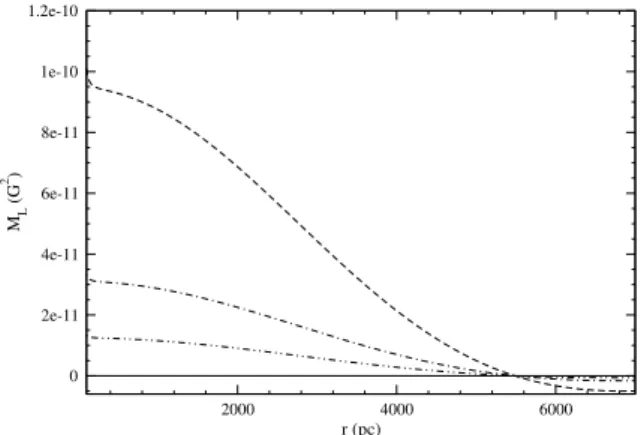
In Fig. 1 we plot the finalML, for different values of
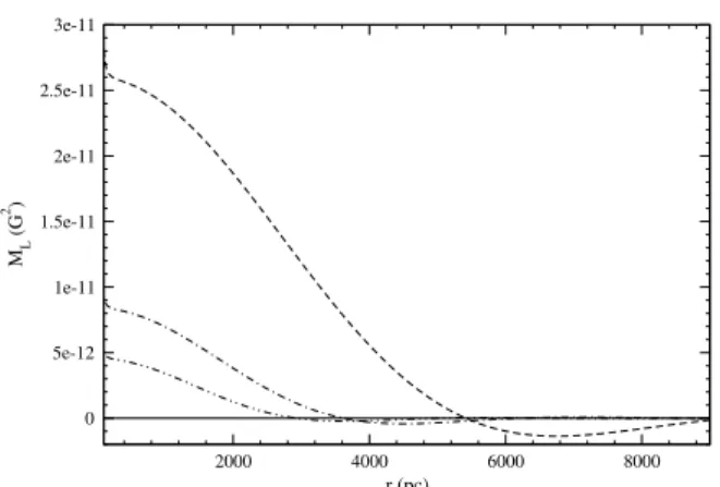
a. We show the finalMLfor different values ofVcin Fig.2. The growth ofML as a function of time for various initial conditions is shown in Fig. 3.
2000 4000 6000 r (pc)
0 2e-11 4e-11 6e-11 8e-11 1e-10 1.2e-10
M
L
(G
2 )
Figure 1. Final magnetic longitudinal correlations,ML (G
2
) as a function of r (pc), for q = 2, p = 1.333, Lc = 83 pc, Ω = 0.98×10⁻¹³s−1andV
c = 98km/s. Three different va-lues foraare shown,a = 3.2×1039
cm3 s g−1(dashed line), 9.7×1039
cm3s g−1 (dash-dotted line) and2.43×1040cm3 s g−1(dash-doubledotted line). We see that the smaller the value of
a, the larger are the magnetic field intensities. The coherence scale remains practically unchanged.
1654 Alejandra Kanduset al.
2000 4000 6000 8000 r (pc)
0 5e-12 1e-11 1.5e-11 2e-11 2.5e-11 3e-11
ML
(G
2 )
Figure 2. Final magnetic longitudinal correlations,ML(G
2
) as a function ofr (in pc), forq = 2,p = 1.33, Lc = 83pc and
a= 3.2×1039
cm3
s g−1. Three different values forV
care shown,
Vc= 30km.s−1(dash-doubledotted line),45km s−1(dash-dotted line) and96km s−1 (dashed line), with corresponding values of Ω = 0.3×10⁻¹³s−1,0.45×10−13s−1and0.96×10−13s−1. We see that for larger values ofVc, larger field intensities and cohe-rence scales are obtained.
1e+05 1e+06 1e+07 t (yrs)
1e-60 1e-54 1e-48 1e-42 1e-36 1e-30 1e-24 1e-18 1e-12
ML
(G
2)
Figure 3. Magnetic longitudinal correlation,ML(G2) as a func-tion oft(yrs), forr0= 112pc and for three different initial values, ML(r0, t= 0) = 1.5×10−
38
G2
(dashed line),1.5×10−47G2 (dash-dotted line) and1.5×10−55G2 (dash-doubledotted line). We usedp= 1.11,q= 2,Lc= 81pc,Ω = 0.75×10⁻¹³s−1,
Vc = 98km s−1,a = 9.76×1038cm3 s g−1. We see that in-dependent of the initial values ofML, saturation occurs at a time
t∼5×10⁶
years whenML1/2∼10−6G.
shown in Figs. 1 and 2, we require the entire time interval 5< z <10for longitudinal correlations to develope.
The age of the universe atz= 10is4.7×108
years. A galaxy at this redshift has already been observed [15]. The star formation rate in this galaxy is observed to be extre-mely high. A high level of turbulence produced by super-novae and star formation can then be assumed to exist al-ready atz ∼ 10and, thus, throughout the redshift interval 5< z <10.
In summary, we found that for a reasonable set of tur-bulent, astrophysical parameters, magnetic fields on the
or-der of10−6
G, as are observed in high redshift objects are generated in less than about 109
years (the time elapsed betweenz∼10andz∼5). They are coherent on scales of
LM ≃3.5−5.4kpc.
Our model for the generation and evolution of magne-tic correlations is relatively simple. Our results, which are preliminary due to the simple evolution equations used, sug-gest that the reionization process of the universe, involving the formation of the first stars, played an important role in determining the features of the magnetic fields detected in high redshift objects.
Acknowledgments
We thank George Morales for useful comments. We ack-nowledge E. Opher for careful proof reading of this manus-cript. This work was partially supported by the Brazilian fi-nancing agency FAPESP (00/06770-2). A.K. acknowledges the FAPESP fellowship (01/07748-3). R. O. acknowledges partial support from the Brazilian financing agency CNPq (300414/82-0).
References
[1] D. Grasso and H. Rubinstein, Phys. Rept.348, 163 (2001); L. M. Widrow, Rev. Mod. Phys.74, 775 (2002)
[2] Ya. B. Zel’dovich, A. A. Ruzmaikin and D. D. Sokoloff, Mag-netic Fields in Astrophysics, (Gordon and Breach, New York, 1983).
[3] K. H. Moffat,Magnetic Field Generation in Electrically Con-ducting Fluids, (Cambridge Univ. Press, Cambridge, 1978)
[4] C. L. Carrilli and R. B. Taylor, ARA&A40, 319 (2002).
[5] A. M. Wolfe, K. M. Lanzetta and A. L. Oren, 1 Astrophys. J. 388, 17 (1992).
[6] K. M. Lanzetta, N. Yahata, S. Pascarelle et al., Astrophys. J. 570, 492 (2002).
[7] A. P. Kazantzev, JETP26, 1031 (1968).
[8] K. Subramanian, Phys. Rev. Lett.83, 2957 (1999).
[9] S. I. Vainshtein and L. L. Kichatinov, J. Fluid Mech.168, 73 (1986),
[10] H. J. V¨olk, U. Klein, and R. Wielebinski, A&A213, L12 (1989).
[11] A. S. Monin, and A. A. Yaglom, A. A.Statistical Fluid Me-chanics, (MIT Press, Cambridge 1975).
[12] S. I. Vainshtein, JETP56, 86 (1982).
[13] Naval Research Laboratory 2002,Plasma Formulary
[14] R.M. Kulsrud and S. W. Anderson, Astrophys. J.396, 606 (1992).