ABSTRACT: This paper concerns a new coupled free wake-CFD method for proper calculation of aerodynamic loads on a two bladed helicopter rotor in hovering light. Loading is computed by solving the three dimensional Euler equations in a rotating coordinate system. However, since direct simulation of the tip vortices and wake requires a very ine grid, the rotor’s wake effects are modeled by a free wake approach and included into the CFD calculation by a transpiration boundary condition at the rotor surface. An inluence coeficient solution method is used to ind the rotor’s wake shape, being steady in a rotating frame. Euler equations are also considered in the form of absolute low variables and solved by a multi grid Jameson’s inite-volume method. The accuracy of the proposed method is illustrated by comparing numerical results to the available experimental results for the pressure distribution on a blade of a model helicopter rotor at different tip Mach numbers.
KEYWORDS: Free wake, Euler equations.
A New Coupled Free Wake-CFD Method
for
Calculation of Helicopter Rotor
Flow-Field in Hover
Hamid Farrokhfal1, Ahmad Reza Pishevar2
INTRODUCTION
he low ield around rotors is inherently complex. In the vicinity of the blade tip, it is highly three dimensional and vortical and it is characterized by non-uniform inlow with blade-vortex interactions and transonic conditions. In hover, the complex’ three dimensional rotor wake has a dominant inluence on the blade loading (Jenny et al., 1968; Clark and Langrebe, 1971; Landgrebe, 1972).
A proper evaluation of the rotor aerodynamic loading has an important role in the analysis and design of helicopter rotor blades. here are two general approaches for simulating the low ield around a rotor and determining its loads. In the irst approach, the inviscid or viscous set of governing equations is solved by a proper Computational Fluid Dynamic (CFD) method (Roberts and Murman, 1985; Chen and McCroskey, 1988; Kramer et al., 1988). Obviously, in this approach, the vortex system near the blade tips and the wake region below the rotor disk must be captured accurately for realistic pressure and load estimations. he computational cost is extremely increased for this approach (Roberts and Murman, 1985; Chen and McCroskey, 1988; Kramer et al., 1988; Ramachandran et al., 1989; Lee and Kwon, 2006; Chen et al., 1987). In the second approach, the tip vortices and the helical wake system are not solved by the CFD calculation and instead, the inluence of strong tip vortices and the geometry of the wake are included by a vortex-wake model.
Solution scheme which use the later idea are often grouped under methods using wake models encompassing the potential flow (Strawn and Caradonna, 1987; Strawn and
1. Malek-Ashtar University of Technology – Isfahan – Iran 2. Isfahan University of Technology – Isfahan – Iran.
Author for correspondence: H. Farrokhfal | Department of Mechanical & Aerospace Engineering | Malek-Ashtar University of Technology – 83145-115 | Shahinshahr – Isfahan – Iran | Email: [email protected]
Tung, 1986; Chang and Tung, 1985; Egolf and Sparks, 1987), the Euler (Sankar et al., 1986, Agarwal and Deese, 1987; Chang and Tung, 1987) and the Navier-Stockes methods (Agarwal and Deese, 1988; Narramore and Vermeland, 1989; Wake and Sankar, 1989; Srinivasan and MacCroskey, 1988). Several approaches have been applied to model the vortical field of rotors. The most famous of these models is the prescribed wake model, which uses experimental data to drive empirical formulas relating the rotor blade geometric parameters and thrust coefficient (C
T) to the vortex’ wake geometry (Kocurek and Tangler, 1976; Landgrebe, 1972; Landgrebe and Cheney, 1972; Landgrebe et al., 1977). These schemes do not correctly model the flow characteristics and their reliance on experimental data causes to not appropriately predict blade loading for a new rotor configuration. Free wake models have been developed in an attempt to overcome these limitations by simulating in details the actual shape and motion of the wake (Crimi, 1965; Landgrebe, 1969; Clark and Leiper, 1970; Sadler, 1971; Johnson, 1980; Johnson, 1981; Summa and Clark, 1979; Summa and Maskew, 1981; Saberi, 1983; Rosen and Graber, 1988). This can be done by finding the geometry of the wake and the strength of tip and sheet vortices, which are modeled by a finite number of vortex line segments. Then, the effect of the vortex-wake is brought into CFD calculation by modifying either the boundary conditions at the blade surface (Sankar et al., 1986, Agarwal and Deese, 1987; Chang and Tung, 1987) or explicitly modifying the blade angle of attack (Wake and Sankar, 1989; Srinivasan and McCroskey, 1988).
There are some advantages for calculating the rotor aerodynamics loads by a coupled wake-CFD method when compared to the direct method. he irst beneit is that accurate enough results can be obtained with signiicant reduction in the computational expense. his is a key factor when a low idelity approach is required for design or multidisciplinary optimization purposes. he second beneit is to relieve the diiculties arisen in meshing the 3-D domains around the rotor. Since the tip region is not computed directly in the CFD calculation, the 3-D grid can be obtained from an assembly of two-dimensional spanwise sectional grids (Caradonna et al., 1984).
The shape of the rotor wake has an intense effect on the aerodynamic performance of a helicopter rotor in hover flight. The present research explains a new interactive wake-CFD solver for calculating the inviscid transonic
flow on a two-bladed rotor in hover flight. In this method, the CFD flow solver is coupled with a free wake model by using the surface transpiration approach, i.e., effects of rotor vortex-wake are included into CFD calculation by using the estimated downwash velocity to modify boundary condition along the blades.
In most of the previously reported works, the induced velocity is computed prior to the CFD analysis by a separate program such as Hover, B-TRIM of McDonnell Douglas Helicopter Company (Agarwal and Deese, 1987), or Host (Benoit et al., 2000). In this work, however, the induced downwash of rotor blades are computed along with the CFD solution and one can interact with it through an iterative procedure. he model is based on a liting line theory, which provides estimation for induced downwash along the blade. In this method, the blade is substituted by a row of square vortex panels in radial direction and, at some location of blade span, a inite number of spiral vortices are shed downwards the disc rotor. hen, the positions of helices are corrected by induced velocities, which are computed by employing the Biot-Savart law and the use of the Basic Curved Vortex Element (BCVE) or Self-Induction Vortex Element (SIVE) elements (Quackenbush et al., 1989). he procedure continues until the shape of the wake converges to a steady state and therefore, the self-induced velocities become from zero up to a tolerance.
hen, the transonic low ield about the rotor is calculated by the solution of the three-dimensional Euler equations on a multi-block structured grid about the blades. However, as mentioned earlier, the three-dimensional grid is constructed from an assembly of 2D grids about the blade sections which is extended only to the blade tip and consists of two blocks that are symmetric in relation to the planform. In this study the inite-volume scheme of Jameson, Schmidt, and Turkel (Jameson et al., 1981) is used to discrete governing equations. he method is reformulated for a rotating coordinate system which is attached to the rotor blades, but equations are finally rewritten in terms of absolute-flow variables. This approach has been used previously by Holmes and Tong (1985) in order to develop an Euler solver for some applications in turbomachinery.
velocity along the blade as a boundary condition. Now, a new bound circulation can be obtained from the lift of each section and therefore, it is possible to improve the wake model accordingly. The procedure is repeated until the blade bound circulation or downwash velocity remains unchanged in two subsequent iterations.
he paper is organized as follows: the methodology used for modeling the rotor wake and tip vortices is explained. Governing equations for CFD calculations are presented and the numerical procedure for discretizing these equations is described. he necessary boundary conditions and the way through which the rotor wake model interacts with the CFD solver are explained. Finally, some illustrative numerical results are presented. Calculations are performed for the low ield of a model helicopter rotor in hover at various collective pitch angles. Comparisons with the experimental data of Caradonna and Tung (1981) are also presented.
ROTOR WAKE MODELING
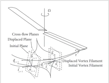
he rotor wake model is based on the proposition that the free wake hover problem possesses a self-preserving state solution when viewed in a rotating frame that is ixed to blades (Bliss et al., 1985). he fundamental idea in the model is that at each point on the rotor wake, when viewed in coordinates rotating with the blade, the velocity contributions due to all efects must be such that there is no convection to change the wake shape. Any velocity component in a plane, normal to the vortex ilament curve, will convect the vortex to a new position, thereby changing the ilament shape (Quackenbush et al., 1989).
Applying the idea, two features of the wake are properly determined: the contraction of the helical wake as it extends in the axial direction below the rotor, and the interaction of the tip vortex of two blades. For modeling the wake, the two curved vortex elements introduced in Bliss et al. (1985) and Baskin et al. (1967) are used. hese elements include the BCVE and SIVE. he BCVE is used in order to compute the velocity induced at any point in the flow field, not on the element itself, and the SIVE is used to evaluate the velocity induced by a vortex ilament on itself, including the efect of distributed vorticity in the bent vortex core. Figure 1 shows two types of vortex elements on a typical helical vortex ilament. he BCVE
is a parabolic arc element positioned between control points whereas the SIVE is a circular arc element passing through each three adjacent control points.
The solution procedure involves a way of reducing the cross low velocity to zero at every collocation point. Figure 2 shows the idea. In order to achieve this goal, for a given arrangement of the free wake collocation points, the net velocity in each cross low plane is computed irst. Next, the efect of small displacements of each collocation point on the velocity at every other collocation point, and the displaced point itself, are determined. hese efects are known as inluence coeicient.
In practice, the solution must be obtained numerically with the wake modeled by using discrete elements. he blade is represented by a set of vortex quadrilaterals in a way that
r j + 2
j + 2 j - 1
j - 2 j - 3
j
Point of Evaluation BCVE
BCVE SIVE
Interpolated Points
BCVE
Ĵ + 2
Ĵ - 1
Ĵ - 2
Figure 1. BCVE and SIVE elements for discretizing wake vortex ilaments.
Cross-flow Planes Displaced Plane
Initial Plane
qj + 1
→
tj + 1
→
bj + 1
→
nj + 1
→
bj
qj →
tj →
→ n
j
r
Displaced Vortex Filament Initial Vortex Filament Ω
→
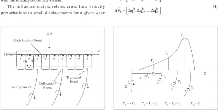
their forward edges are located at the quarter chord line of the blade and the distance of their at edges from the blade trailing edge is also one-fourth of the local chord. he vortex ilaments of sheet vortex and the tip vortex are shed from the points on the at legs of these panels, and the panels including the shed points are in the form of truncated vortices, as shown in Fig. 3.
Figure 4 shows a schematic of a typical load distribution on a rotor blade. It is assumed that the corresponding wake consists of four ilaments, whose strengths are deined as shown in the igure. he locations of the release point are also computed from the Batchelor principle (Batchelor, 1967) as:
(1)
where is the distance of the release point of the vortex ilament from the center of rotation.
he velocity contribution of each individual vortex element is determined analytically using the Biot-Savart law. he total velocity vector at a collocation point includes the local self-induction efect (SIVE), the contributions from the rest of the wake (BCVE’s), the velocity induced by the bound circulation on the rotor blades, and the swirl velocity component associated with the rotating coordinate system.
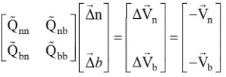
The influence matrix relates cross flow velocity perturbations to small displacements for a given wake
configuration. This matrix can be used to predict the set of collocation point displacements, which will eliminate the cross flow velocity. If the free wake location is described in terms of the positions of N collocation points, and the normal and binormal cross flow velocity components at the ith point are denoted by and , respectively; then the N-dimensional vectors based on these velocity components are defined as:
(2)
he free wake solution is achieved when a set of collocation
point locations is found, such as .
he amplitudes of small displacements on the ith collocation point in the local normal and binormal directions are denoted by and . From these, changes of displacement vectors are deined as:
(3)
and the normal and binormal velocity component changes, associated with the above displacement vectors, are:
(4)
Blade Control Point
Trailing Vortex CollocationPoints
Truncated Panel
Ω Z
Z
Z ZV
Ω Υ
1
Υ
1 = - Γ1 Υ2 = Γ1 - Γ2 Υ3 = Γ2 - Γ3 Υ4 = Γ3 Υ2
Υ3
Υ 4 Γ
2
Γ3
Γ 1
Figure 3. Schematic of the quadrilateral vortex panels of the blade.
he velocity change vectors can be related to the change of displacement vectors through the inluence coeicient sub matrices, namely:
(5)
For instance, the sub matrix gives the changes in normal velocity due to binormal displacements. hese matrices must be evaluated numerically. To obtain zero net cross low velocity, the collocation point displacements must be chosen so that the velocity changes cancel the net cross low velocity,
namely, = and = , which means solving
the following matrix equation for and :
(6)
Since the wake problem is actually nonlinear, this process must be repeated several times.
A free wake analysis involves only a inite number of turns of free vortex. Beyond the free wake region is an adaptive mid wake which completes the contraction process. he inal part is also a semi-ininite helical wake having constant radius and constant pitch based on the momentum theory. he location and geometry of the adaptive mid wake depend on the position of the last points in the near section of the wake. In other words, the last points of near wake section are the beginning points of the mid-section, and ater the mid-section the wake model is continued with the far section as shown in Fig. 5.
From the conservation of mass low within the contracting mid wake and by applying the momentum theory, it is possible to drive the boundary shape of the mid wake (Bliss et al., 1985) as:
(7)
where and are the axial and radial locations of the last free wake points, and is the inal contraction radius. In hover light, the radial contraction exponent is given by:
(8)
where is the azimuth location of the last free wake point. When calculating two-bladed rotors, the solution is symmetric from one blade to the next blade. his symmetry allows the induced efect of the second blade on the primary wake to be expressed in terms of the corresponding efect of the primary wake on the second blade.
Once all the different effects have been computed and summed, the resultant velocity vectors at each collocation point are expressed in the blade ixed reference frame. hese resultant velocity vectors are solved into the local normal and binormal directions in order to obtain the cross low velocity components and their changes, associated with point displacements. he velocity changes are normalized by the unit displacement magnitudes to obtain the inluence coeicients. hese coeicients, as described earlier, are used to predict how the collocation points should be displaced in order to reduce the velocity components in the cross low planes. he obtained result at this stage is not the inal solution due to the nonlinear nature of the problem. herefore, starting from an initial wake shape, the solution procedure is repeated with a proper relaxation factor in quasi linear steps to improve the convergence rate (Bliss et al., 1984).
he Initial wake shape can be estimated from a contracted wake model with a contraction ratio of = 0.85, where is the radius of the contracted far section of the wake.
Z
Γ
Ω
Near Wake Last Free Wake Point
Adaptative Mid Wake
Momentum Theory Far Wake x
y0
(y0)
y rb
Γf
he circulation distribution is also obtained from an approach explained by Baskin et al. (1967); in other words, equating the 2-D lit coeicient of blade section to the lit coeicient obtained from the Kutta-Joukowski theorem. As a result, a system of linear algebraic equation is obtained by deining the sought circulation. By knowing the circulation, the convergent shape of the wake is computed as explained in the previous section. Finally, at the end, the distribution of the downwash on blade surface is computed. his downwash is then fed to the CFD solver to include the compressibility efect and to correct the circulation. he circulation at this stage is computed from the integration of the pressure ield around the blade sections and by using the Kutta-Joukowski theorem. With this new distribution of the circulation, the free wake solver provides a new downwash distribution and this process is iterated until a convergent solution for the downwash is attained.
GOVERNING EQUATIONS
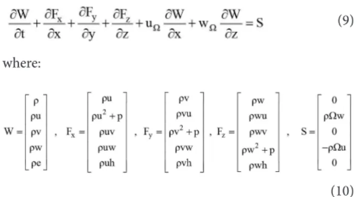
Let (u,v,w) denote the absolute velocity components in the rotating Cartesian coordinate system (x,y,z), as shown in Fig. 6. Compressible Euler equations can be formulated as (Agarwal and Deese, 1987):
(9)
where:
(10)
and ( , , ) denotes the rotational velocity components:
(11)
Deining the lux vector and rotational speed vector as:
and:
where ( , , ) are the unit vectors in the (x, y, z) coordinate system, Eq. (9) can be written as:
(12)
Equation (12) can be solved by the inite-volume method described in the next section.
NUMERICAL METHOD
In order to apply the inite-volume method, Eq. (12) is written in its integral form as:
(13)
The computational domain is meshed by a multiblock structured hexahedral grid. Applying Eq. (13) to a typical (i,j,k) cell, for a cell center algorithm, we obtain a system of ordinary diferential equations as:
(14)
where is the cell volume, represents the net convectional lux out of the cell, and and are rotational luxes out of each cell. We rewrite Eq. (14) as:
X
Y
Ω
(15)
he convective luxes can be determined by a second order central scheme. However, the resultant scheme is not dissipative, and therefore, undamped oscillations at odd and even mesh points can be developed during the computation. In order to suppress the tendency for odd-even decoupling, and to prevent the appearance of oscillations in regions containing severe pressure gradients near shock waves and stagnation points, the inite-volume scheme is modiied by the addition of artiicial dissipative terms as below:
(16)
where denotes the dissipative luxes. Jameson et al. (1981) have established that an efective form of dissipative terms for lows with discontinuities is a blend of second and fourth diferences, with coeicients which depend on the local pressure gradient. herefore, dissipative terms are written as follows:
(17)
Where:
(18)
and is deined as:
(19)
Δx denotes the forward diference operator
and ò(2) and ò(4) are adaptive coeicients deined as:
(20)
(21)
(22)
Typical values of the constants κ(2) and κ(4) are κ(2) = 0.5, κ(4) = 1/64. Also, is deined as:
(23)
where CFL is the courant number and ( , , ) are the spectral radii for each cell:
(24)
a is the speed of sound and (U, V, W) are the contavariant velocities:
(25)
(Ur, Vr, Wr) are the components of relative velocity obtained from:
(26)
( , , ),( , , ) and ( , , ) are the metrics of transformation for computational coordinates ( , , ). Other dissipation terms, DyWy,j,k and DzWy,j,k, in Eq. (17), are calculated in an analogous manner.
Equation (16) can be integrated in time by a multistage Runge-Kutta scheme. he conserved variables are updated to the new time level n+1 as:
where α
m = 1, and D(w
(k))=β(k) D(W(n+1,k))+(1-β(k))D(W(k-1)). For a ith-stage scheme the coeicients are given as:
(28)
In this work a local time stepping and residual smoothing procedure is also used in order to improve the convergence rate.
BOUNDARY CONDITIONS
Special care must be given to the boundary conditions when solving Euler equations for rotor blades of a helicopter by a coupled free wake-CFD method. he computational domain, as shown in Fig. 7, is a cylinder with radius of 1.5 times the blade span. A far-ield boundary condition is applied at the outer surface of the cylinder and also at the blade tip plane. In addition to that, at the root of the blade, the symmetry boundary condition is applied where z axis is along the blade span. At the solid surface of the blade, the transpiration condition is applied to take into account the efects of the wake in the CFD calculations. In this method, the usual velocity to the blade surface is calculated so that it exactly cancels out the efect of the wake normal downwash to the surface.
he boundary condition at the blade surface must be modiied in order to include the wake efects. For invicid calculations, this becomes:
(29)
where is the wake induced velocity and is the normal unit vector of the blade surface. hus, the induced velocity is used to modify the conventional tangency of velocity vector at the solid surface. Also, the luxes of density and the enthalpy at the solid surface are modiied accordingly to meet the new boundary condition.
It is interesting to note that, for a computational region covering only a portion of the rotor disk, the efect caused by the other rotor blades and the low outside the inite computational region are incorporated into the calculation by employing the above transpiration velocity technique if the efects of other blades are included in the induced downwash velocity.
he treatment of the far-ield boundary condition is based on the concept of Riemann invariants for a one-dimensional flow normal to the boundary (Jameson and Baker, 1983). Let subscripts ∞ and e denote far-field values and values extrapolated from the interior cells adjacent to the boundary, respectively, and let Vn and a be the velocity component normal to boundary and to the speed of sound (a). If the low in the far ield is subsonic, ixed and extrapolated Riemann invariants are introduced as:
(30)
Which are corresponding to incoming and outgoing waves. hese invariants may be added and subtracted to obtain:
(31)
At an outflow boundary, we extrapolate the tangential components of velocity, which results in:
(32)
And for an inlow boundary, the tangential components are those of the free stream:
(33)
Block No. 2 Block No. 1 Y
Z X
he procedure is completed by extrapolating the entropy at an outlow boundary S = Se or setting it equal to its free stream value at inlow boundary S = S∞. he density, energy and pressure can then be calculated from a and s.
RESULTS
In this section some illustrative examples are presented as to demonstrate the capability of the proposed method for predicting the aerodynamic load and the low ield of a model helicopter rotor in hover state at various tip speeds. he rotor is a two bladed rotor with an aspect ratio of 6, which are untwisted and have rectangular planform with the NACA-0012 airfoil section. he experiments on this rotor have been presented by Caradonna and Tung (1981) at the NASA Ames Research Center. Computations are performed on a two-block mesh with 141570 nodes, on a personal computer. Figure 7 shows the computational domain which is symmetric in relation to the blade planform.
Five orders of magnitude reduction in the density residual are considered as convergence criteria. However, in most simulations for a Courant number of 2.0, the convergence criteria is not met in less than 1,600 time steps for the irst iteration of the free wake model, and it is reduced to around 800 steps for the next iterations. Some of the results are discussed in the following sub-sections.
NON-LIFTING CASE
For this case, the free wake model is switched off and only the CFD calculation is performed. Pressure distribution on the blade upper and lower surfaces is shown in Fig. 8 for a tip Mach number of Mt = 0.52 and zero collective angle. Except near the tip, the agreement between the Euler calculation and the experimental data is obvious. The discrepancy near the tip can be caused by boundary conditions. However, the difference between numerical and excremental results is not significant.
LIFTING CASES
As stated before, for this case, the rotor downwash is irst calculated by modeling the blade vortices with the BCVE vortex elements. hen, the efect of the wake and tip vortices is fed
into the CFD solver and a new bound circulation is calculated from the sectional lit. Finally, a new iteration is started by correcting the shape of the wake and its strength according to the new bound circulation. he procedure is continued until the induced downwash velocity converges to a steady form. For the liting cases, calculations are performed for ive blade tip Mach numbers and in four diferent collective angles. For these simulations, the bound vortex is modeled by 32 vortex rings. In the near ield part, the tip vortex is modeled by 3 turns of a helical vortex ilament, each turn composed by six BCVE elements. he pitch of helix is initially set to in this region, where the initial CT is estimated from a collective angle by using the rotor momentum theory. he sheet vortices are also modeled by 4 ilaments, each helical ilament has 2 turns and each turn has six basic vortex elements. he mid part of the wake consists of 8 turns of helical ilaments with the same axial pitch as the near wake ilaments, i.e., . Also the far part of the wake consists of 50 turns with an axial pitch, which is twice the value used in the mid part.
For these simulations the number of iterations required for the convergence of induced downwash velocity is less than 300 iterations for a known circulation distribution in the free wake solver, and the number of iterations for achieving a steady distribution of downwash velocity from the combined free wake-CFD solver at low collective angles is six while it is reduced to less than 4 iterations for higher angles.
he sectional lit coeicient and the circulation distribution obtained from these calculations are shown in Fig. 9. he non-dimensional circulation (experimental or numerical) is deined as:
(34)
where C1 is the section lit coeicient at z radial station. he circulation shown in these igures is non-dimensioned byR2Ω, where Ω is the rotational velocity of the rotor and R is the rotor radius. As can be seen from these igures, the agreement with the experimental data is satisfactory. he thrust and inviscid power coeicients have also been computed and presented in Table 1. Comparison reveals that coeicients have good coincidence with experimental data (Caradonna and Tung, 1981) for all collective angles.
the free wake model and the CFD solver is depicted in Fig. 10. It should be pointed out that through this iterative process, the compressibility efects in the tip region of the blades are
included into the free wake model. Figure 10 shows that the downwash, or circulation distribution, is converged to a steady form in a few iterations.
-0.5
-0.4 -0.2 0 0.2 0.4 0.5
z/r = 0.5
1 0
Cp
x/c
-0.5
-0.4 -0.2 0 0.2 0.4 0.5
1 0
Cp
x/c
z/r = 0.68
-0.5
-0.4 -0.2 0 0.2 0.4 0.5
1 0
Cp
x/c
z/r = 0.8
-0.5
-0.4 -0.2 0 0.2 0.4 0.5
1 0
Cp
x/c
z/r = 0.89
-0.5
-0.4 -0.2 0 0.2 0.4 0.5
z/r = 0.96
Euler Free Wake Calculations Experimental Data 1
0
Cp
x/c
Figure 8. Pressure distribution in non-lifting case, Mt = 0.52, θ
Table 1. The computed thrust and power coeficients and comparison with experimental data.
Collective Angle
(degree) Tip Mach No.
Thrust Coeficient×103
(Computed)
Thrust Coeficient×103
(Experimental)
Power Coeficient×104
(Computed)
2.0 0.830 0.615 0.690 0.935
5.0 0.815 2.253 2.190 1.769
8.0 0.439 4.655 4.590 3.120
8.0 0.877 4.606 4.730 4.262
12.0 0.794 7.730 7.920 7.941
0,04
Mt = 0.749, t0 = 12
Mt = 0.877, t0 = 8
Mt = 0.439, t0 = 8
Mt = 0.815, t0 = 5
Mt = 0.830, t0 = 2 Experiment Calculation
0,02
0
0.4 0.6 0.8
z/R
N
o
m. D
in. C
ir
cu
la
ti
o
n
0.6 0.5 0.4
Experiment Mt = 0.794, T0 = 12
Mt = 0.877, T0 = 8
Mt = 0.439, T0 = 8
Mt = 0.815, T0 = 5
Mt = 0.830, T0 = 2
Calculation
0.3 0.2 0.1 0 -0.1
0.4 0.6 0.8
z/R
Cl
Figure 9. Lift coeficient and circulation distribution at various tip Mach numbers and collective angles.
0.03
0.02
0.01
0
-0.01
0.2 0.4 0.6 0.8
N
o
n
D
in
. C
ir
cun
la
ti
o
n
z/R
Colletive = 0.8 deg. Mt = 0.877
itr = 2
itr = 1 itr = 3
itr = 4
0.03
0.02
0.01
0
-0.01
0.2 0.4 0.6 0.8 1
N
o
n
D
in
. D
ow
n
w
a
sh
z/R
Colletive = 0.8 deg. Mt = 0.877
itr = 1
itr = 2 itr = 3
-2
-1.5
-1
-0.5
0
0.5
1
1.5
-0.4 -0.2 0 0.2 0.4
Cp
x/c
z/R = 0.5
-2 -2.5
-1.5
-1
-0.5
0
0.5
1
1.5
-0.4 -0.2 0 0.2 0.4
Cp
x/c
z/R = 0.68
-2 -2.5
-1.5
-1
-0.5
0
0.5
1
1.5
-0.4 -0.2 0 0.2 0.4
Cp
x/c
z/R = 0.80 -1.5
-1
-0.5
0
0.5
1
1.5
-0.4 -0.2 0 0.2 0.4
Cp
x/c
z/R = 0.89
-1.5 -2
-1
-0.5
0
0.5
1
1.5
-0.4 -0.2
Euler Free Wake Calculations
Experimental Data
0 0.2 0.4
Cp
x/c
z/R = 0.96
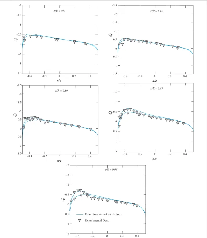
Figure 11. Pressure distribution on a lifting rotor in hover, Mt = 0.830, θ
c = 2deg.
Pressure distribution is shown in Figs. 11-15 for diferent tip Mach numbers and collective angles from 2 to 12 degrees. As shown in these
-1.5 -2
-1
-0.5
0
0.5
1
1.5
-0.4 -0.2 0 0.2 0.4
Cp
x/c
z/R = 0.5
-1.5 -2 -2.5
-1
-0.5
0
0.5
1
1.5
-0.4 -0.2 0 0.2 0.4
Cp
x/c
z/R = 0.68
-1.5 -2 -2.5
-1
-0.5
0
0.5
1
1.5
-0.4 -0.2 0 0.2 0.4
Cp
x/c
z/R = 0.80
-1.5 -2
-1
-0.5
0
0.5
1
1.5
-0.4 -0.2 0 0.2 0.4
Cp
x/c
z/R = 0.89
-1.5 -2
-1
-0.5
0
0.5
1
1.5
-0.4 -0.2
Euler Free wake Calculations
Experimental Data
0 0.2 0.4
Cp
x/c
z/R = 0.96
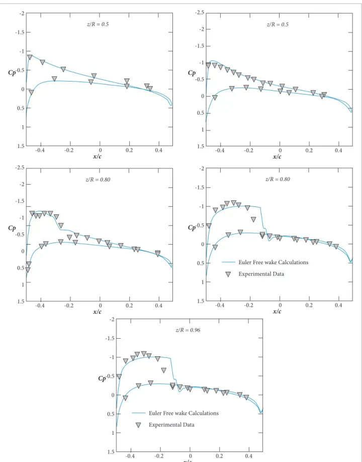
Figure 12. Pressure distribution on a lifting rotor in hover, Mt = 0.815, θ
c = 5deg.
The flow solver can also be run in a full multi-grid (FMG) mode, which accelerates the process of convergence. Figure 16 shows the results obtained by applying the FMG approach in
-1.5 -2
-1
-0.5
0
0.5
1
1.5
-0.4 -0.2 0 0.2 0.4
Cp
x/c z/R = 0.5
-1.5 -2 -2.5
-1
-0.5
0
0.5
1
1.5
-0.4 -0.2 0 0.2 0.4
Cp
x/c z/R = 0.68
-1.5 -2 -2.5
-1
-0.5
0
0.5
1
1.5
-0.4 -0.2 0 0.2 0.4
Cp
x/c z/R = 0.68
-1.5 -2
-1
-0.5
0
0.5
1
1.5
-0.4 -0.2 0 0.2 0.4
Cp
x/c z/R = 0.89
-1.5 -2
-1
-0.5
0
0.5
1
1.5
-0.4 -0.2 0
Euler Free Wake Calculations
Experimental Data
0.2 0.4
Cp
x/c z/R = 0.96
Figure 13. Pressure distribution on a lifting rotor in hover, Mt = 0.439, θ
-1.5 -2
-1
-0.5
0
0.5
1
1.5
-0.4 -0.2 0 0.2 0.4
Cp
x/c
z/R = 0.5
-1.5 -2 -2.5
-1
-0.5
0
0.5
1
1.5
-0.4 -0.2 0 0.2 0.4
Cp
x/c
z/R = 0.5
-1.5 -2 -2.5
-1
-0.5
0
0.5
1
1.5
-0.4 -0.2 0 0.2 0.4
Cp
x/c
z/R = 0.80
-1.5 -2
-1
-0.5
0
0.5
1
1.5
-0.4 -0.2 0
Euler Free wake Calculations
Experimental Data
0.2 0.4
Cp
x/c
z/R = 0.80
-1.5 -2
-1
-0.5
0
0.5
1
1.5
-0.4 -0.2 0
Euler Free wake Calculations
Experimental Data
0.2 0.4
Cp
x/c
z/R = 0.96
Figure 14. Pressure distribution on a lifting rotor in hover, Mt = 0.877, θ
-1.5 -2
-1
-0.5
0
0.5
1
1.5
-0.4 -0.2 0 0.2 0.4
Cp
x/c
z/R = 0.5
-1.5 -2.5
-2
-1
-0.5
0
0.5
1
1.5
-0.4 -0.2 0 0.2 0.4
Cp
x/c
z/R = 0.68
-1.5 -2.5
-2
-1
-0.5
0
0.5
1
1.5
-0.4 -0.2 0 0.2 0.4
Cp
x/c
z/R = 0.80
-1.5 -2
-1
-0.5
0
0.5
1
1.5
-0.4 -0.2 0 0.2 0.4
Cp
x/c
z/R = 0.89
-1.5 -2
-1
-0.5
0
0.5
1
1.5
-0.4 -0.2 0
Euler Free Wake Calculations
Experimental Data
0.2 0.4
Cp
x/c
z/R = 0.96
Figure 15. Pressure distribution on a lifting rotor in hover, Mt = 0.794, θ
-1.5
-1
-0.5
0
0.5
1
-0.4 -0.2 0 0.2 0.4
Cp
x/c
z/R = 0.80
-1.5
-1
-0.5
0
0.5
1
-0.4 -0.2 0 0.2 0.4
Cp
x/c
z/R = 0.89
-1.5
-1
-0.5
0
0.5
1
-0.4 -0.2 0
Euler Free Wake Calculations
Experimental Data
0.2 0.4
Cp
x/c
z/R = 0.96
Figure 16. Pressure distribution on a lifting rotor in hover obtained from FMG approach,Mt = 0.877, θ
c = 8deg, AR = 6.0.
CONCLUSION
A new coupled free wake-CFD methodology for evaluation of aerodynamic loads on a helicopter rotor in hovering condition was introduced. In this approach, the Euler equations are solved in a rotating coordinate system and the rotor wake efects are modeled by a free wake approach and included into the CFD solver by a transpiration boundary condition at the blade surface.
he obtained results from this approach for the pressure distribution on the blade surface are promising; the performance
REFERENCES
Agarwal, R.K. and Deese, J.E., 1987, “Euler Calculation for Flowield of a Helicopter Rotor in Hover” AIAA, Journal of Aircraft, Vol.24, No.4, pp. 231-238. doi: 10.2514/3.45431.
Agarwal, R.K. and Deese, J.E., 1988, “Navier-Stokes Calculations of
the Flow ield of a Helicopter Rotor in Hover”, AIAA 26th Aerospace
Sciences Meeting, Paper 88-0106. doi: 10.2514/6.1988-106.
Baskin, V.E., Vildgrube, L.S., Vozhdayev, Y.S. and Maykapar, G.I., 1967, “Theory of Lifting Airscrew”, NASA TTF-823.
Batchelor, G.K., 1967, “An Introduction to Fluid Dynamics”, Cambridge University Press.
Benoit, B., Dequim, A.M., Kampa K., Grünhagen, W., Basset, P.M. and Gimonent B., 2000, “HOST, a General Helicopter Simulation tool for Germany and France”, In Proceeding of: American Helicopter Society, 56th Annual Forum and Technology Display, Virginia Beach, VA.
Bliss, D.B., Wachspress, D.A. and Quackenbush, T.R., 1984, “A New Methodology for Free Wake Analysis Using Curved Vortex Elements”, Continuum Dynamics, Inc. Report No. 84-6.
Bliss, D.B., Wachspress, D.A. and Quackenbush, T.R., 1985, “A New Approach to the Free Wake Problem for Hovering Rotors”, Proceedings of the 41st Annual Forum of the American Helicopter Society, Fort Worth, TX, pp. 463-477.
Caradonna, F.X. and Tung, C., 1981, “Experimental and Analytical Studies of a Model Helicopter Rotor in Hover”, Vertica, Vol. 5, pp. 149-161.
Caradonna, F.X., Tung, C. and Desopper, A., 1984, “Finite Difference Modeling of Rotor Flows Including Wake Effects”, Journal of the American Helicopter Society, Vol. 29, No. 2, pp. 26-33(8). doi: 10.4050/JAHS.29.26.
Chang, L.C. and Tung, C., 1985, “Numerical Solution of the Full Potential Equation for Rotors and Oblique Wings Using a New Wake Model”, AIAA Paper 85-0268.
Chang, L.C., and Tung, C., 1987, “Euler Solution of the Transonic Flow
for a Helicopter Rotor”, AIAA 25th Aerospace Sciences Meeting, Paper
87-0523. doi: 10.2514/6.1987-523
Chen, C.L. and McCroskey, W.J., 1988, “Numerical Simulation of Helicopter Multi-Bladed Rotor Flow”, AIAA, Aerospace Sciences Meeting, Paper 88-0046.
Chen, C.S., Velkoff, H.R. and Tung, C., 1987, “Free-Wake Analysis of a Rotor in Hover”, AIAA Paper 87-1245.
Clark, D.R and Landgrebe, A.J., 1971, “Wake and Boundary Layer Effects in Helicopter Rotor Aerodynamics,” AIAA 4th Fluid and Plasma Dynamics Conference, AIAA paper No. 71-581.
Clark, D.R. and Leiper, A.C., 1970, “The Free Wake Analysis: A Method for the Prediction of Helicopter Rotor Hovering Performance”, Journal of the American Helicopter Society, Vol. 15, No. 1.
Crimi, P., 1965, “Theoretical Prediction of the Flow in the Wake of a Helicopter Rotor”, Cornell Aeronautical Laboratory, Report CAL BB-1994-S.
Egolf, T.A. and Sparks, S.P., 1987, “A Full Potential Flow Analysis with Realistic Wake Inluence for Helicopter Rotor Airload Prediction”, NASA CR-4007.
Holmes, D.G. and Tong, S.S., 1985, “A Three-Dimensional Euler Solver for Turbomachinery Blade Rows”, Journal of Engineering for Gas Turbines and Power, Transactions of ASME, Vol. 107, No. 2, pp. 258-264. doi: 10.1115/1.3239705.
Jameson, A. and Baker, T.J., 1983, “Solution of Euler Equations for Complex Conigurations”, AIAA Paper 83-1929.
Jameson, A., Schmidt, W. and Turkel, E., 1981, “Numerical Solution of the Euler Equations by Finite Volume Methods Using Runge-Kutta
Time-Stepping Schemes”, AIAA, 14th Fluid and Plasma Dynamics
Conference, Paper 81-1259.
Jenny, D.S., Olson, J.R. and Landgrebe, A.J., 1968, “A Reassessment of Rotor Hovering Performance Predic tion Methods”, Journal of American Helicopter Society, Vol. 13, No. 2, pp. 1-26. doi: 10.4050/JAHS.13.1.
Johnson, W., 1980, “Helicopter Theory”, Princeton University Press.
Johnson, W., 1981, “Development of a Comprehensive Analysis for Rotorcraft - I. Rotor Model and Wake Analysis”, Vertica, Vol. 5, No. 2, pp. 99-129.
Kocurek, J.D. and Tangler, J.L., 1976, “A Prescribed Wake Lifting Surface Hover Performance Analysis”, Journal of the American Helicopter Society, Vol. 22, No. 1, pp. 24-35. doi: 10.4050/JAHS.22.24.
Kramer, E., Hertel, J. and Wagner, S., 1988, “Computa tion of
Subsonic and Transonic Helicopter Rotor Flow using Euler Equations”, Vertica, Vol. 12, No. 3, pp. 279-291.
Landgrebe, A.J., 1969, “An Analytical Method for Predicting Rotor Wake Geometries”, Journal of the American Helicopter Society, Vol. 14, No. 4, pp.20-32(13). doi: 10.4050/JAHS.14.20.
Landgrebe, A.J., 1972, “The Wake Geometry of a Hovering Helicopter Rotor and its Inluence on Rotor Performance”, Proceedings of the 28th Annual National Forum of the American Helicopter Society, Journal of the American Helicopter Society, Vol. 17, No. 4, pp. 3-15(13). doi: 10.4050/JAHS.17.3.
Landgrebe, A.J. and Cheney, M.C., 1972, “Rotor Wakes-key to Performance Prediction”, AGARD Conference Proceedings No. 111 on Aerodynamics of Rotary Wings.
Landgrebe, A.J., Mofitt, R.C. and Clark, D.R., 1977, “Aerodynamic Technology for Advanced Rotorcraft-Part I”, Journal of the American Helicopter Society, Vol. 22, No. 2, pp. 21-27. doi: 10.4050/ JAHS.22.21.
Lee, S.W. and Kwon, O.J., 2006, “Aerodynamic Shape Optimization of Hovering Rotor Blades in Transonic Flow Using Unstructured Meshes”, AIAA Journal, Vol. 44, No. 8, pp. 181-1825. doi: 10.2514/1.15385.
Narramore, J.C. and Vermeland, R., 1989, “Use of Navier-Stokes Code to Predict Flow Phenomena Near Stall as Measured on a 0.658-Scale V-22 Tilt-rotor Blade”, AIAA Paper 89-1814.
Quackenbush, T.R., Bliss, D.B. and Wachspress, D.A., 1989, “New Free-wake Analysis of Hover Performance Using a New Inluence Coeficient Method”, NASA CR 4309, Journal of Aircraft, Vol. 26, No. 12, pp. 1090-1097. doi: 10.2514/3.45885.
Roberts, T.W. and Murman, E.M., 1985 “Solution Method for a Hovering Helicopter Rotor Using the Euler Equations”, AIAA Paper 85-0436.
Rosen, A. and Graber, A., 1988, “Free Wake Model of Hovering Rotors Having Straight or Curved Blades”, Proceedings of the International Conference on Rotorcraft Basic Research, Journal of the American Helicopter Society, Vol. 33, No. 3, pp. 11-19(9). doi: 10.4050/ JAHS.33.11.
Saberi, H.A., 1983, “Analytical Model of Rotor Aerodynamics in Ground Effect”, NASA CR 166533.
Sadler, S.G., 1971, “Development and Application of a Method for Predicting Rotor Free Wake Positions and Resulting Rotor Blade Airloads”, NASA CR 1911 and CR 1912.
Sankar, N.L., Wake, B.E. and Lekoudis, S.G., 1986, “Solution of the Unsteady Euler Equations for Fixed and Rotor Wing Conigurations”, Journal of Aircraft, Vol. 23, No. 4, pp. 283-289. doi: 10.2514/3.45301.
Srinivasan, G.R. and McCroskey, W.J., 1988, “Navier- Stokes
Calculations of Hovering Rotor Flow Fields”, Journal of Aircraft, Vol. 25, No. 10, pp. 865-874. doi: 10.2514/3.45673.
Strawn, R.C. and Caradonna, F.X., 1987, “Conservative Full-Potential Model for Unsteady Transonic Rotor Flows”, AIAA Journal, Vol. 25, No. 2, pp. 193-198. doi: 10.2514/3.9608.
Strawn, R.C. and Tung, C., 1986, “The Prediction of Transonic Loading on Advancing Helicopter Rotors”, NASA TM-88238.
Summa, J.M. and Clark, D.R., 1979, “A Lifting-Surface Method for Hover/Climb Airloads”, Proceedings of the 35th Annual National Forum of the American Helicopter Society, Washington, D.C., USA.
Summa, J.M. and Maskew, B., 1981, “A Surface Singularity Method for Rotors in Hover or Climb”, USAAVRADCOM TR 81-D-23.