A Brief Comment on the Dynamical Behavior of a …
J. of the Braz. Soc. of Mech. Sci. & Eng. Copyright © 2005 by ABCM April-June 2005, Vol. XXVII, No. 2 /205
A. Fenili
and L. C. Gadelha de Souza
Divisão de Mecânica Espacial e Controle Instituto Nacional de Pesquisas Espaciais (INPE) 12227-010 São José dos Campos, SP. Brazil [email protected] [email protected]
J. M. Balthazar
Istituto de Geociências e Ciências Exatas Departamento de Estatistica, Matemática Aplicada e Computação (UNESP) CP 178 13500-230 Rio Claro, SP. Brazil and Departamento de Projeto Mecânico (UNICAMP) 13084-971Campinas, SP. Brazil [email protected]
L. C. S. Góes
Departamento de Engenharia Mecânica Aeronáutica Instituto Tecnológico de Aeronáutica (ITA) 12228-900 São José dos Campos, SP. Brazil [email protected]
A Brief Comment on the Dynamical
Behavior of a Forced Nonlinear
Slewing Beam: 1. Superharmonic
Resonance
This paper describes the dynamical behavior of a nonlinear flexible beam (cubic nonlinearities considered) connected to a dc motor (responsible for the slewing motion) when the angular displacement of the slewing axis and its derivatives are considered to be of a harmonic type and the system is excited near a resonance (present due to the nonlinear contribution).
Keywords: Slewing structure, nonlinear vibrations, resonance, multiple scale method
Introduction
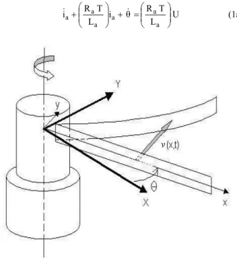
The idea in this paper is to present some analytical results on the investigation about nonlinear mechanical systems composed by (or including) rotating flexible beam-like structures (lightweight robotic manipulators, satellite antennas, solar panels...) harmonically excited. A schematic of the slewing flexible structure studied here is shown in figure 1.1
The dynamic analysis developed in this paper considers a nonlinear flexible beam-like structure clamped to an oscillating hub or actuator (harmonically driven), which represents the beam excitation.
The governing equations of motion are presented in the perturbed form (Fenili, 2000); (Fenili 2004a); (Fenili, 2004b). In this case, all the nonlinearities plus the structural damping are considered as small perturbations around a known linear system.
The amplitude and phase equations of the perturbed problem are derived and its steady state behavior investigated in the vicinity of a resonant cases (Hayashi, 1964; Schmidt and Tondl, 1986; Cunningham, 1958; Drazin, 1994).
Governing Equations of Motion: N Modes
Equations (1a), (1b) and (1c) are the nondimensional perturbed governing equations of motion for the nonlinear slewing flexible beam-like structure driven by a dc motor (Fenili, 2000). Equations (1a) and (1b) are the governing equations of the actuator (dc motor: Equation (1a) represents the governing equation for the electric
Paper accepted May, 2005. Technical Editor: Atila P. Silva Freire.
current and Equation (1b) represents the governing equation for the angular displacement of the motor axis) and Equation (1c) is the governing equation of the time component, qi, of the transverse
displacement of the flexible beam.
U L
T R
θ
i L
T R i
a a a
a a
a ⎟⎟
⎠ ⎞ ⎜⎜ ⎝ ⎛ = + ⎟⎟ ⎠ ⎞ ⎜⎜ ⎝ ⎛
+
(1a)
A. Fenili et al
/ Vol. XXVII, No. 2, April-June 2005
ABCM
206 ⎟ ⎟ ⎠ ⎞ ⎜ ⎜ ⎝ ⎛ + = ⎟⎟ ⎠ ⎞ ⎜⎜ ⎝ ⎛ + = = − + ) I (I L T K K I I T c 0 i θ θ motor shaft a 2 b t 2 motor shaft v 1 a 2 1 f f f f (1b)
(
)
(
)
0 q q q Γ q q q q q Λ q q θ λ q q θ q θ q µ θ α q w q N 1 i N 1 j N 1k ijk i j k N 1 i N 1 j N 1
k ijk i j k j k N
1 i
N 1
j ij i j ij i j N
1 i i i 2 2 2 = ⎥ ⎥ ⎦ ⎤ ∑ ∑ ∑ ⎢ ⎢ ⎢ ⎢ ⎢ ⎣ ⎡ ∑ ∑∑ + + + ∑ ∑℘ − − ∑ + ∈ + + + = = = = = = = = = A A A A A A A A A A (1c)
The boundary conditions are given by:φA(0)=0, φ′A(0)=0, φ′′A(1)=0 and φ ′′′A(1)=0.
In Equations (1a) and (1b), Ra represents the armature resistance, T
represents the period of the first natural frequency of the beam, La
represents the armature inductance, cv represents the motor internal
damping, Ishaft represents the inertia of the connecting motor-beam
shaft, Imotor represents the inertia of the motor, Kt represents the
torque constant and Kb represents the back e.m.f. constant. In
Equation (1c):
( ) ( )
∫ φ′ ξφ′ ξ ξ=
= x
ji j
i
ij 0 d R
R (1d)
( )
∫ φ ξ ξ −
= 1
x d
Vi i (1e)
( ) ( )
[
]
η∫ ∫ φ′ ξφ′ ξ ξ −
= η d d
Sij 1x 0 i j (1f)
( ) ( )
∫ φ′ ξφ ξ ξ −
= 1 x
ij d
W i j (1g)
∫ φ =
α 1
0x Adx
A (1h)
1 ] d ) 1 ( 2 1
[∫01 2 ⎟ −
⎠ ⎞ ⎜
⎝
⎛ φ′φ + − φ ′′φ =
βiA x i A x i A x (1i)
℘ijA=∫01
(
2RijφA−2φ ′′iVjφA−2φ′iφjφA)
dx (1j)∫ ⎟
⎠ ⎞ ⎜
⎝
⎛− φ +φ ′′ φ +φ′φ φ =
λ 1
0 2R V d
1 x j i j i ij
ijA A A A (1k)
(
)
∫ φ ′′φ + φ′φ =
Λ 1
0Sjk i Rjk i dx
ijkA A A (1l)
(
)
∫ ⎥ ⎥ ⎥ ⎥ ⎥ ⎥ ⎥ ⎦ ⎤ ⎢ ⎢ ⎢ ⎢ ⎢ ⎢ ⎢ ⎣ ⎡ φ φ′′ + φ φ′ φ φ′ + φ φ′′ φ′′ φ′′ + φ φ ′′′ φ′′ φ′ = Γ 1 0 2 4 4 d W ) 8780 . 1 ( 2 3 8780 . 1 3 xwj i j k ij k j i k j i ijk A A A A A (1m)
Where E represents the Young modulus, I represents the inertia of the beam cross section around the neutral axis, L represents the beam length, φA represents each one of the flexural vibration modes of the beam and wA represents the frequencies associated to these modes.
Governing Equations of Motion: 1 Mode
Consider now that the behavior of the flexible structure can be represented by only one flexural mode (the first). The governing equations given by (1a) to (1c) are reduced to (Fenili et al, 2004a):
U L T R θ i L T R i a a a a a a ⎟⎟ ⎠ ⎞ ⎜⎜ ⎝ ⎛ = + ⎟⎟ ⎠ ⎞ ⎜⎜ ⎝ ⎛ + (2a) ⎟ ⎟ ⎠ ⎞ ⎜ ⎜ ⎝ ⎛ + = ⎟⎟ ⎠ ⎞ ⎜⎜ ⎝ ⎛ + = = − + ) I (I L T K K I I T c 0 i θ θ motor shaft a 2 b t 2 motor shaft v 1 a 2 1 f f f f (2b)
[
]
0 3 1 1111 2 1 1111 2 1 1 1111 2 1 111 1 1 111 1 11 2 1 2 1 1 2 1 1 = Γ + Λ + Λ + + θ λ − θ ℘ − β θ + µ ∈ + θ α + + q q q q q q q q q q q w q k (2c)and the same boundary conditions as before.
As can be seen again for the set of Equations (2a) to (2b), the governing equations for the dc motor does not depend on the equation for q1. In this sense, the behavior of the variable θ (and its
derivatives) is known beforehand.
In this work, the prescribed angular displacement is considered a harmonic function, with frequency Ω, of the type:
(
ei t e i t)
i C t
C Ω = Ω − −Ω
= θ 2 1 ) sin( (3)
where the amplitude of excitation, C, is considered equal to 1 (Fenili et al, 2003).
Amplitude and Phase Modulation Equations
Equation (2c) is a nonlinear perturbed governing equation of motion and its analytical solution can be found by using some perturbation technique such as the multiple scale method (Nayfeh and Mook, 1979; Nayfeh, 1981; Nayfeh, 1993).
The main idea here is to eliminate all the possible conditions under which the desired analytic solution of Equation (2c) is unboundedin time.
The amplitude of vibration increases in time as a direct consequence of the presence of secular and small divisor terms in this solution. Several different cases can be found associated with this unbounded condition of the system solution (in other words, the system resonance’s).
There is a pair of modulation equations (amplitude and phase) for each one of the critical cases and they can be studied separately.
Only the particular case w1 3 1
Ω≈ is studied here.
The fixed-point (steady state) solutions are the wanted ones and the focus in this kind of analysis. The original governing equations (2c) are reduced to the ones that represent the system in this desired condition.
A Brief Comment on the Dynamical Behavior of a …
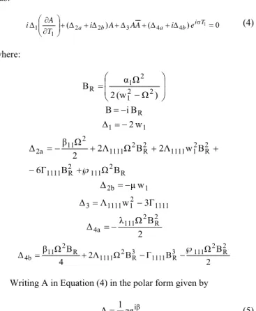
J. of the Braz. Soc. of Mech. Sci. & Eng. Copyright © 2005 by ABCM April-June 2005, Vol. XXVII, No. 2 /207 and substituting in the O (∈2) equation and to bounded solution one
has:
0 ) (
)
( 1
4 4 3 2 2 1
1 ⎟⎟+ ∆ +∆ +∆ + ∆ +∆ =
⎠ ⎞ ⎜⎜ ⎝ ⎛ ∂
∂
∆ iσT
b a b
a i A AA i e
T A
i (4)
where:
⎟ ⎟ ⎠ ⎞ ⎜
⎜ ⎝ ⎛
− =
)
Ω
(w 2
Ω α
B
2 2 1
2 1 R
R B i B=−
1
1 2w
∆ =−
R 2 111 2 R 1111
2 R 2 1 1111 2
R 2 1111 2
11 2a
B
Ω
B 6Γ
B w 2Λ B
Ω
2Λ 2
Ω ∆
℘ + −
+ +
+ − =
1
2b µw
∆ =−
1111 2
1 1111
3 Λ w 3Γ
∆ = −
2 B
Ω λ
∆ 111 2 2R 4a =−
2 B Ω B
Γ B Ω 2Λ 4
B Ω
∆ 3 111 2 2R
R 1111 3 R 2 1111 R
2 11 4b
℘ − −
+ =
Writing A in Equation (4) in the polar form given by
i ae 2 1
A= (5)
and separating the new equation in real and imaginary part, amplitude (a) and phase (β) modulation equations of the system
response for the case w1 3 1
Ω≈ (superharmonic resonance) has the
form shown in Equations (6).
) cos(σo
∆
2∆ ) sen(σe
∆
2∆ a
∆ ∆
a 1
1 4b 1
1 4a
1
2b − − − −
=
′ (6a)
) sen(σe
∆
2∆
) cos(σo
∆
2∆ a 4∆
∆
a
∆ ∆
a
1 1
4b
1 1
4a 3
1 3
1 2a
− −
+ − +
+ = ′
(6b)
or, in autonomous form:
cos
∆
2∆ sen
∆
2∆ a
∆ ∆
a
1 4b
1 4a
1
2b − −
=
′ (7a)
sen
∆
2∆ cos
∆
2∆ a 4∆
∆
a
∆ ∆
a
σ
a
1 4b
1 4a 3
1 3
1
2a − − +
− =
′ (7b)
where
β − σ =
γ T1 (8)
Frequency Response Function
Squaring both sides of Equations (9a) and (9b) and adding them one obtains:
0
∆
)
∆
4(∆ a
∆ ∆ ∆ ∆ ∆
2∆
σ σ
a 2∆
∆ σ
2∆
∆ ∆
a 16∆
∆
2 1
2 4b 2 4a 2
2 1 2 2b 2 1 2 2a
1 2a 2
4
1 3 2
1 3 2a 6 2 1 2 3
= ⎥ ⎥ ⎦ ⎤ ⎢
⎢ ⎣
⎡ +
− ⎥ ⎥ ⎦ ⎤ ⎢
⎢ ⎣ ⎡
+ + −
+
+ ⎥ ⎥ ⎦ ⎤ ⎢
⎢ ⎣ ⎡
− +
⎥ ⎥ ⎦ ⎤ ⎢ ⎢ ⎣ ⎡
(10)
which represents the damped frequency response function for the
case w1
3 1
Ω≈ . The parameter a in equation (10) represents the
steady state amplitudes of the system response.
Some Numerical Results in the Resonant Region Around
1
w 3 1
Figures 2 to 4 illustrate the steady state vibration amplitudes for different values of the excitation frequency (Ω) in the
neighborhood of w1 3 1
.
In these figures, the broken lines represent unstable solutions and the full line represents stable steady state solutions. The stable solutions are the ones the real system will realize (maintain).
The values of the parameters used in the numerical simulations are given in Table 1.
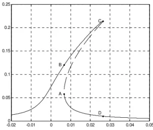
In Figure 2, the length of the beam is varied and the frequency response curve is plotted for each one of the cases.
Figure 3 shows the influence of the beam structural damping,
µ
, over the amplitude of vibration of the beam in steady state.The higher the value of this parameter the closer the behavior of the frequency response curve for the perturbed system is to the linear frequency response curve obtained by doing ∈=0. It is evident that the damping can act in the sense of killing all the nonlinear effects on the system.
Figure 4 shows the upward jump, obtained by increasing the frequency of excitation, and the backward jump, obtained by decreasing the frequency of excitation.
The type of jump that will occur depends on the direction one goes over the curve. This jump phenomenon is an as signature of a nonlinear system.
Table 1. Parameter values used in the simulations( young Modulus( aluminum-beam) and density( aluminium): beam.
Parameter Value Unit
Beam length 1.0 m
Beam cross section 0.0008 X 0.0100 m (X m)
Young modulus 0.7 1011 N/m
Density: beam 2700 kg/m3
-A. Fenili et al
/ Vol. XXVII, No. 2, April-June 2005
ABCM
208
-0.020 -0.01 0 0.01 0.02 0.03 0.04 0.05 0.05
0.1 0.15 0.2 0.25
σ
a
A B
C
D
Figure 2. Frequency response curves for different values of the beam length, L. (dimensional µ=0.0010Kg/s).
-0.02 -0.015 -0.01 -0.005 0 0.005 0.01 0.015 0.02 0.025 0.03 0
0.05 0.1 0.15 0.2 0.25
σ
a
L=0.8m
L=0.9m
L=1.0m
Figure 3. Frequency response curves for w1
3 1
Ω≈ and L=1.0 m. The
values of µ considered here are.
-0.020 -0.01 0 0.01 0.02 0.03 0.04 0.05 0.05
0.1 0.15 0.2 0.25
σ
a
Figure 4. Backward jump (A → B) and forward jump (C → D) for µ = 0.00010 Kg/s.
Conclusions
The numerical simulations presented in this work discuss the dynamical behavior of a nonlinear flexible beam when clamped to the axis of a dc motor and excited near a superharmonic resonance by a prescribed harmonic angular displacementθ.
The influence of the structural damping of the beam over the frequency response curves is also investigated.
By increasing the value of this parameter one brings the peak of the frequency response curves to the origin of the adopted reference frame and the shape of the curve approximates the one for linear case. It was also verified that the same behavior obtained with the increasing of µ could be verified for increasing values of L, the beam length. In future works we will discuss another resonance’s. This is the first work of a series of them.
An extension to another rsonances will be done in next future.
Acknowledgements
The authors thank to FAPESP and CNPq both Brazilian Researches Funding Agencies.
References
Cunningham, W. J., “Introduction to Nonlinear Analysis”, McGraw-Hill Book Company, 1958.
Drazin, P. G., “Nonlinear Systems”, Cambridge Texts in Applied Mathematics, Cambridge University Pres, 1994.
Fenili, A., “Modelagem matemática e análise dos comportamentos ideal e não ideal de estruturas flexíveis de rastreamento e aplicações em engenharia mecânica” , Ph.D. Dissertation , Faculdade de Engenharia Mecânica of the Universidade Estadual de Campinas, Campinas, São Paulo, Brazil, 2000.
Fenili, A., Souza, L.C.G., Góes, L.C.S., Balthazar, J. M., “Investigation of Resonance on a Harmonically Forced Non-Linear Slewing Beam”, AIAC 2003 - Australian International Aerospace Congress (incorporating the 14th National Space Engineering Symposium), Brisbane, Australia, 29 julho a 1 de agosto, 2003.
Fenili, A., Balthazar, J. M., “ mathematical modeling of a beam-like flexible structure in slewing motion assuming nonlinear curvature”, Journal of Sound and Vibration, 282 p. 543-552, 2004.
Fenili, A., Balthazar, J. M., “ some remarks on nonlinear vibrations of ideal and non-ideal slewing flexible structures”, Journal of Sound and Vibration, 268, p. 800-841, 2005.
Hayashi, C., “Nonlinear Oscillations in Physical Systems”, McGraw-Hill Book Company, 1964.
Nayfeh, A. H., Mook, D. T., “Nonlinear oscillations”, John Wiley and Sons, Inc., New York, 1979.
Nayfeh, A. H., “Introduction to Perturbation Techniques”, John Wiley and Sons, Inc., 1981.
Nayfeh, A. H., “Problems in Perturbation”, John Wiley and Sons, Inc., 1993.