doi: 10.1590/0101-7438.2015.035.01.0091
SPECIAL LOTTERY DRAWINGS – ANALYSIS OF AN UNCONVENTIONAL INVESTMENT OPPORTUNITY
Jaques Deivinson da Silva Castello
1and Armando Zeferino Milioni
2*Received August 31, 2013 / Accepted June 14, 2014
ABSTRACT.Quina Loto is one of the most popular lottery games in Brazil. Prizes are paid as a per-centage of each drawing’s revenues. After deductions and taxes, 34% of the revenues are destined for the payments of prizes on each drawing, 29% divided among winners and 5% saved in order to contribute for the major prize of the special drawing held annually, in June 24th. Due to the low expected return on in-vestment, lotteries are widely regarded as a bad investment decision. Experience, however, shows that the special drawing might be an exception. In this paper we provide a thorough analysis of a theoretical invest-ment in the special drawing of 2013, considering players’ behavior, lesser prizes earnings, effects of the own investment in the jackpot, probabilities of sharing the prizes and outcomes covering methods. Finally, we compare our conclusions against the result of the lottery on June 24th, 2013.
Keywords: Lotto, Wallenius random variable, investment decision, applied probability, applied statistics.
1 INTRODUCTION
Loto III, widely known as Quina, was created in 1994 and today is the 3rdmost popular lottery game in Brazil, in terms of revenues. Drawings are held 6 times a week, from Monday to Satur-day, and, in each of them, 5 numbers are randomly selected out of a pool of 80 numbers. Players, on the other hand, are allowed to select either 5, 6 or 7 numbers, paying, respectively, R$ 0.75, R$ 3.00 or R$ 7.50 for each of these bets. Prizes are paid as a percentage of each drawing’s revenues. After deductions and taxes, 34.1% of the revenues are destined for the payments of prizes on each drawing – 10.8% divided among players with 5 correct matches, 7.7% among those with 4 matches and 11.0% among those with 3. The remaining 4.6%, in turn, are saved in order to contribute for the major prize of the special drawing held annually, in June 24th, known asQuina de S˜ao Jo˜ao(see CEF, 2011 and 2012).
Due to the low expected return on investment, 29.5% for regular drawings as seen above, lot-teries are widely regarded as a bad investment decision. Experience, however, shows that the
*Corresponding author.
1300 Liberty Ave, apt 1013, Pittsburgh – PA. E-mail: [email protected]
special drawing might be an exception – first prize winners in 2012 drawing were awarded with R$ 12.7 million each while one could, theoretically, afford to play all the possible combinations for R$ 8.6 million.
The objective of this paper is to provide a thorough analysis of a theoretical investment in the special drawing of 2013, considering players’ behavior, lesser prizes earnings, effects of the own investment in the jackpot, probabilities of sharing the prizes and outcomes covering methods.
2 DEVELOPMENTS
2.1 Odds of winning
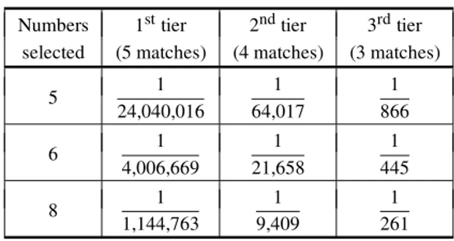
Quina follows a fairly simple lottery model and players are considered winners when their bet contains 5, 4 or 3 correct matches with the 5 numbers drawn in the raffle, hereby referred as 1st, 2nd and 3rdprize tiers’ winners, respectively. Odds of winning, for each of the prize tiers, follow a hypergeometric distribution which varies according to the amount of numbers selected, as illustrated in Table 1. It is important to notice that differently from other lottery games in Brazil, minor prizes winners receive a single prize even if they choose to play with multiple bets (6 or 7 numbers selected).
Table 1– Odds of winning per prize tier.
Numbers 1sttier 2ndtier 3rdtier selected (5 matches) (4 matches) (3 matches)
5 1
24,040,016
1 64,017
1 866
6 1
4,006,669
1 21,658
1 445
8 1
1,144,763
1 9,409
1 261
2.2 Economical imbalance of bets
One of the main contributing factors for the positive expected return on investment is the eco-nomical imbalance of bets. As mentioned before, players are allowed to select 5, 6 or 7 numbers on each bet, paying, respectively R$ 0.75, R$ 3.00 or R$ 7.50. Chances of winning however do not follow the same proportion. While those who choose to play with 5 numbers cover one single output for each bet, those who play 7 numbers cover a total of7
5
=21 possible outputs, but
Table 2– Outputs vs. price comparison.
Numbers Outputs
Price Outputs/ selected covered price ratio
5 1 R$ 0.75 1.33
6 6 R$ 3.00 2.00
7 21 R$ 7.50 2.80
2.3 Number of players per kind of ticket
Given that the payout for gamblers varies according to the amount of numbers selected, it is im-portant to understand how many of them will choose to play 5, 6 or 7 numbers. This information, however, is not disclosed by CEF, the lottery manager, and estimation methods are necessary to derive an answer.
For the period analyzed, information is available for the number of winners in each of the prize tiers and for the total revenues with bets. LetN5,N6andN7represent the number of bets con-taining 5, 6 or 7 numbers, the number of winners in the analyzed period for each of the tiers can be estimated, with errorε, as:
⎡ ⎢ ⎢ ⎢ ⎢ ⎢ ⎢ ⎢ ⎣ 1 24,040,016 1 4,006,669 1 1,144,763 1 64,017 1 21,658 1 9,409 1 866 1 445 1 261 ⎤ ⎥ ⎥ ⎥ ⎥ ⎥ ⎥ ⎥ ⎦ ⎡ ⎢ ⎣ N5 N6 N7 ⎤ ⎥ ⎦= ⎡ ⎢ ⎣ 200 45,461 2,986,809 ⎤ ⎥ ⎦+ε
To offset the difference in the magnitude between tiers, this equation can be rewritten as:
⎡ ⎢ ⎢ ⎢ ⎢ ⎢ ⎢ ⎢ ⎣ 1
200×24,040,016
1 200×4,006,669
1 200×1,144,763 1
45,461×64,017
1 45,461×21,658
1 45,461×9,409 1
2,986,809×866
1 2,986,809×445
1 2,986,809×261
⎤ ⎥ ⎥ ⎥ ⎥ ⎥ ⎥ ⎥ ⎦ ⎡ ⎢ ⎣ N5 N6 N7 ⎤ ⎥ ⎦= ⎡ ⎢ ⎣ 1 1 1 ⎤ ⎥ ⎦+ε
′
Observing that the total revenues should add up to a total of 0.75N5+3.00 N6+7.50N7 = 2,605,662,369.00, above equation can be solved by using the ordinary least squares method to minimizeε′Tε′. Results suggest that 88.55% of bets contain 5 numbers, while 7.26% contain 6 and 4.17% contain 7 numbers.
These results also allow us to derive an average price for the ticket,c, which is further used for calculating the number of tickets sold based on the sales in reais, so that:
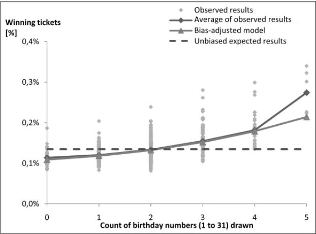
2.4 Evidence of players’ bias
While one could assume players select numbers randomly among those available in the pool, studies suggest that ‘birthday numbers’ (1 to 31, referring to the day of the month) tend to be more popular than other numbers (Thaler & Ziemba, 1988). This trend becomes evident when the percentage of winning tickets is plotted against the count of birthday numbers drawn among the winning numbers, as shown in Figure 1.
0,0% 0,1% 0,2% 0,3% 0,4%
0 1 2 3 4 5
Winningtickets
[%]
Countofbirthdaynumbers(1to31)drawn
Resultadosobservados Médiadosvaloresobservados Valoresperado(semviés) Observed results
Average ofobservedresults Unbiased expectedresults
Figure 1– % of winning tickets in 3rdprize tier vs. count of ‘birthday numbers’.
The same trend can be observed on Table 3, where the numbers are ordered according to the frequency that players pick them (CEF, 2012).
Table 3– Numbers ordered according to the frequency that they are chosen.
70 61 50 66 60 76 38 71 31 58 40 51 68 69 30 46 57 52 41 63 73 80 39 59 64 36 74 77 67 65 75 20 42 78 72 22 49 62 32 79 29 47 28 45 44 56 21 23 54 53 43 48 2 1 16 34 15 37 33 19 55 8 35 27 26 24 18 12 17 11
25 6 14 3 10 4 9 7 5 13
2.5 Probability under bias conditions
In order to understand how players’ bias affects the distribution of the number of winners it is first necessary to calculate the odds of winning for a biased ticket, given a certain amount of birthday numbers are drawn among the winning ones. Supposing a player selectsnbbirthday
numbers amongn numbers played, the probability that he or she getskcorrect matches giventb
out of the 5 numbers drawn are also birthday numbers is given by:
p(k)=
k
r=0
hypg(r; tb, nb, 31)·hypg(k−r; 5−tb, n−nb, 49)
where:
hypg(k; t,n,m)= n
k
m−n t−k
m t
2.6 Mathematical modeling of players behavior
To model the population of players mathematically, two distinct categories were considered. Namely:
• Category A: fractionαof players who select numbers randomly. The probabilityϕA that
nbbirthday numbers are picked among thennumbers played is given by a straightforward
hypergeometric distribution.
ϕA(nb; ;n)=hypg(nb; n, 31, 80)
• Category B: fractionβ =(1−α)of players who have a bias towards birthday numbers. For these players, birthday numbers were considered to beωtimes more likely to be picked over non-birthday numbers, which leads to a Wallenius’ non-central hypergeometric dis-tribution (in the context of this paper, Wallenius’ disdis-tribution was preferred over Fisher’s to reflect the sequential, competitive, process when of the choice of numbers) for the number of birthday numbers picked, which means that the probabilityϕBthatnbbirthday numbers
are picked amongnnumbers played is given by:
ϕB(nb; n)=wnchypg(nb; n,31, 80, ω)
which is calculated recursively (Fog, 2008) by using the fact that:
wnchypg(k; t, n, m, ω) =wnchypg(k−1; t−1, n, m, ω)
× (n−k+1)ω
(n−k+1)ω+m−t−n+k
+wnchypg(k; t−1, n, m, ω)
restricted to:wnchypg(0; 0,n, m, ω)=1
wnchypg(k; t, n, m, ω)=0; ∀k<0
wnchypg(k; t, n, m, ω)=0; ∀k>t
Considering the 3rd prize tier to minimize random variation, the expected number of winning bets consideringtbbirthday numbers are drawn in the raffle, E(W3), can be calculated as the sum of the expected number of winning bets for each of the categories of players and for each kind of bet within these categories. More specifically, considering the entire data set, the total number of winners whentbbirthday numbers were drawn, given that the ticket sales added up to
R(tb)can be estimated as:
E(W3)= A c ×
88.55%· 5
nb=0
[αϕA(nb; 5)+βϕB(nb; 5)]
× 3
k=0
hypg(k; tb, nb, 31)·hypg(3−k; 5−tb, 5−nb, 49)
+7.26%· 6
nb=0
[αϕA(nb; 6)+βϕB(nb; 6)]
× 3
k=0
hypg(k; tb, nb, 31)·hypg(3−k; 5−tb, 6−nb, 49)
+4.19%· 7
nb=0
[αϕA(nb; 7)+βϕB(nb; 7)]
× 3
k=0
hypg(k; tb, nb, 31)·hypg(3−k; 5−tb, 7−nb, 49)
Fraction of tickets Fraction of tickets Individual probability of containing containingnb winning a 3rdtier prize
nnumbers birthday numbers under bias conditions
Stressing this expression numerically by using Frontline Systems SolverAdd-In for Microsoft Excel, it is possible to determineα andωso that the difference between the observed and theoretical results is minimal in a least-squared sense, which yields:
α=69.0%
ω=2.000
0,0% 0,1% 0,2% 0,3% 0,4%
0 1 2 3 4 5
Winningtickets
[%]
Countofbirthdaynumbers(1to31)drawn
Resultadosobservados Médiadosvaloresobservados Valoresperado(ajustado) Valoresperado(semviés) Observed results
Average ofobservedresults BiasͲadjusted model Unbiased expectedresults
Figure 2– Gordon et al., 1995 and Gr¨undlich, 2004.
2.7 The covering problem
As previously shown, tickets with 6 and 7 numbers have an economical advantage over 5 numbers tickets, due to their higher output coverage for each real invested. However, while covering all of the 24,040,016 possible 5-uple outcomes with tickets containing 5 numbers is a trivial problem, doing so with tickets containing 6 or more numbers is a combinatorial problem, known as ‘the covering problem’, which still has no closed solution (Burger et al., 2003a and 2003b). The problem is that, as the number of bets made rise, it becomes increasingly harder (and eventually impossible) to find a bet whose outputs do not overlap those of bets already made (see Gordon et al., 1995; Gr¨undlich, 2004 and Du Plessis, 2010).
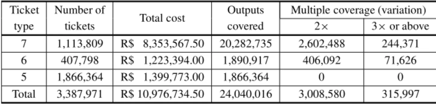
Hence, to determine a solution which approaches the optimal, a heuristic greedy algorithm was used. The algorithm starts by running through all the possible 7 number combinations and select-ing those in which none of the 21 outputs covered overlap those of combinations already selected. Then, the no-overlap requirement is relaxed to allow 1 overlap among the 21 outputs covered and the procedure runs through all the possible 7 number combinations once more. Eventually, when the procedure would allow 7 overlaps per bet, it turns out that 6 number tickets with no output overlap become more advantageous for covering purposes and the algorithm then runs through all the 6 number combinations in a similar fashion.
Table 4– Covering algorithm output.
Ticket Number of
Total cost Outputs Multiple coverage (variation)
type tickets covered 2× 3×or above
7 1,113,809 R$ 8,353,567.50 20,282,735 2,602,488 244,371 6 407,798 R$ 1,223,394.00 1,890,917 406,092 71,626 5 1,866,364 R$ 1,399,773.00 1,866,364 0 0 Total 3,387,971 R$ 10,976,734.50 24,040,016 3,008,580 315,997
Results show that, while one could assume all of the possible outcomes could be covered with 1,144,763×R$ 7.50=R$ 8,585,722.50, a 28% higher investment is, in fact, required to do so. On the other hand, several of the outputs are covered twice or more, which yields a 12.5% (1.3%) chance of having two (three) winning tickets in the 1stprize tier.
2.8 Expected jackpot – fixed part
The jackpot for the special drawing of June 24 can be divided in two parts, a fixed part, which doesn’t depend on the number of players, and a variable part, which grows proportionally to the drawing’s revenues. The fixed part is composed by the fraction saved on the preceding regular drawings over a 1-year period,AS, and by an eventual 1sttier prize rolled over from the previous
drawing, in case it had no winners,AR.
To estimate the prize resulting from the fraction saved in regular drawings, the special drawing of 2012 was used as a proxy. For the 63 first regular drawings which contributed for the special drawing of 2012, the revenues added up to a total of R$ 307,686,432.75 and the amount saved in all the preceding regular drawings totaled R$ 73,426,979.04. The revenues of the first 63 regular drawings contributing for the special drawing of 2013, on the other hand, added up to a total of R$ 325,800,059.25 so it is expected that the amount saved for this drawing totals:
AS=
325,800,059.25
307,686,432.75×R$ 73,426,979.04=R$ 77,749,655.41
An eventual rolled over prize from the previous drawing may also add up to this total. For the data analyzed the rolled over prize averages:
AR =R$ 985,456.76
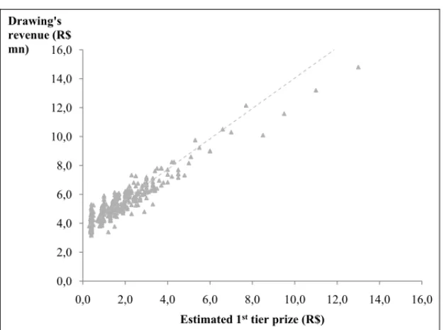
2.9 Expected revenue
Assuming this same coefficient holds true for special drawings, one may infer the revenue for a drawingRi based on the previous drawing revenue Ri−1 and on the 1sttier prize released by CEF for each of them,JiandJi−1:
Ri −Ri−1=0.892×(Ji−Ji−1)
0,0 2,0 4,0 6,0 8,0 10,0 12,0 14,0 16,0
0,0 2,0 4,0 6,0 8,0 10,0 12,0 14,0 16,0
Drawing's revenue (R$ mn)
Estimated 1sttier prize (R$)
Figure 3– Revenues vs. announced 1sttier prize for regular drawings.
Assuming that CEF’s estimates for the 1sttier prize is equal to the actual prize and knowing that 15.41% of the revenues are reverted to the prize, this equation can be rewritten as:
Ri −Ri−1=0.892×((AR+AS+15.41%×Ri)−Ji−1)
Ri =
0.892×(AR+AS−Ji−1)+Ri−1 1−0.892×15.41%
Plugging in AR and AS calculated in the previous section and knowing that for the previous
special drawingJi−1=R$ 88,000,000.00 and Ri−1=R$ 101,013,611.25, the equation yields:
Ri =R$ 107,523,938.41
which suggests a total number of tickets sold NT =89,884,645, N5 =79,589,643 of which containing 5 numbers,N6=6,529,069 containing 6 numbers andN7=3,765,934 containing 7.
When the own investment is includedRi becomes:
2.10 Jackpot breakdown
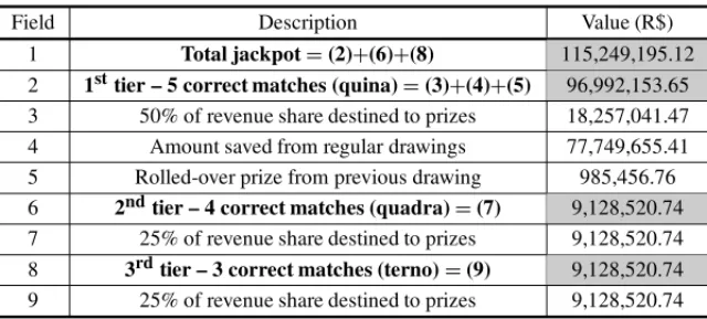
Considering the fixed part of the jackpot and the revenue of drawing, it is possible to break the jackpot down between each of the prize tiers, according to the rules defined by CEF, as shown in Table 5.
Table 5– Jackpot breakdown after income tax by prize tier.
Field Description Value (R$)
1 Total jackpot=(2)+(6)+(8) 115,249,195.12 2 1sttier – 5 correct matches (quina)=(3)+(4)+(5) 96,992,153.65 3 50% of revenue share destined to prizes 18,257,041.47 4 Amount saved from regular drawings 77,749,655.41 5 Rolled-over prize from previous drawing 985,456.76 6 2ndtier – 4 correct matches (quadra)=(7) 9,128,520.74 7 25% of revenue share destined to prizes 9,128,520.74 8 3rdtier – 3 correct matches (terno)=(9) 9,128,520.74 9 25% of revenue share destined to prizes 9,128,520.74
2.11 Prize sharing
One of the key factors to take into account when analyzing lottery investments is the likelihood to share prizes with other players. Given a certain number of other players N also take part in the game with a probabilitypof winning, the number of winners follows a binomial distribution in whichnis the number of trials andpis the success probability for each trial.
When N is large and psmall, as in our case, this distribution strongly converges to a Poisson distribution with parameterλ = N p(Simons, 1971), which keeps the useful property that the addition of Poisson distributed variables is also a Poisson distributed variable.
Considering that players have a bias towards selecting birthday numbers the parameterλvaries significantly with the amount of numbers from 1 to 31 drawn,tb. For instance, considering the
population of players who select a total ofn numbers per bet, the expected number of players withk correct matches, λ, consideringtb birthday numbers were drawn in the raffle is given
by the sum of the parameters for the subgroups of this population which selected nb birthday
numbers or:
λ(k,n; tb)=Nn n
nb=0
[αϕA(nb; n)+βϕB(nb; n)]
×
k
r=0
hypg(r; tb, nb, 31)hypg(k−r; 5−tb, n−nb, 49)
Table 6 summarizes the values forλ(k,n; tb). Hence, knowing that the probability thattb
birth-day numbers will be drawn in the raffle is calculated ashypg(tb, 5, 31, 80), and if Xk is the
random variable that describes the number of third party winners withkcorrect matches, then:
p(Xk =x)=
5
tb=0
hypg(tb, 5, 31, 80)
7
n=5
(λ(k,n; tb))xeλ(k,n;tb)
x!
Table 6– Expected number of winners per prize tier and bet type –λ.
k-correct n-bet Nn-number tb– ‘birthday numbers’ drawn (probability of occurrence)
matches type of players 0 (8%) 1 (27%) 2 (36%) 3 (22%) 4 (6%) 5 (1%)
5 79,589,643 2.5 2.7 3.1 3.9 5.6 9.0
5 6 6,529,069 1.2 1.3 1.5 1.9 2.7 4.4
7 3,765,934 2.5 2.7 3.1 3.9 5.5 8.8
Total 89,884,645 6.2 6.7 7.7 9.7 13.9 22.3 5 79,589,643 960 1,044 1,191 1,445 1,870 2,549
4 6 6,529,069 234 254 290 351 452 612
7 3,765,934 311 338 385 465 597 805
Total 89,884,645 1,504 1,635 1,866 2,261 2,918 3,966 5 79,589,643 74,298 80,732 90,289 103,923 122,497 146,792
3 6 6,529,069 11,893 12,920 14,432 16,570 19,453 23,179 7 3,765,934 11,709 12,716 14,187 16,248 18,996 22,507 Total 89,884,645 97,900 106,367 118,909 136,741 160,946 192,478
2.12 Return on investment per tier
As previously seen, the covering algorithm ensures at least one 1sttier winning ticket among the bets, with a 12.5% chance of having two winning tickets and 1.3% of having 3 or more. LetQ be the random variable that describes the number of 1sttier winning tickets among the ones bet andY5the one that describes the associated return on investment associated with tickets with 5 correct matches. Considering that the 1sttier jackpot stands atJ5, the probability of obtaining a return on investmentY5=yis:
p(Y5=y)= ∞
q=1
p(Q=q)·p
X5=q
J
5 y −1
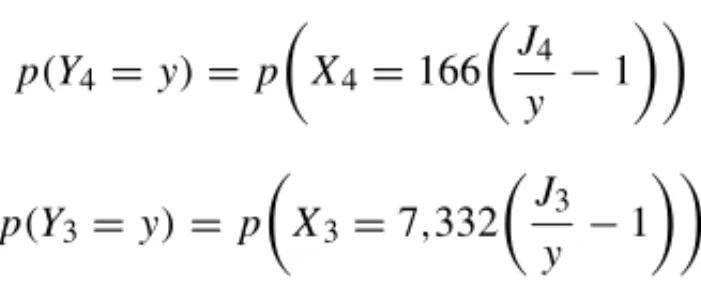
Similarly, but now considering that the number of winning tickets for the 2nd and 3rdtiers are fixed and given by:
• 2ndtier: 1,866,364× 1
64,107+407,798× 1
21,658+1,113,899× 1
9,409=166
• 3rdtier: 1,866,364× 1
866+407,798× 1
445+1,113,899× 1
The distribution of returns obtained from lesser prizes is:
p(Y4=y)=p
X4=166
J
4 y −1
p(Y3=y)=p
X3=7,332
J
3 y −1
The probability mass functions for the return in each of the tiers are illustrated in Figure 4.
Figure 4– Probability mass functions of return on investment in R$ millions for (a) 1st prize tier, (b) 2ndprize tier and (c) 3rdprize tier (consolidated in groups of 100 data points).
It is worth noticing how the 1sttier prize outweighs the minor prizes and the peaks in the distri-butions arising from the effect of the birthday numbers.
2.13 Consolidated return on investment
The total return on investment, Y, is calculated as the sum of the returns obtained from each prize tier,Y =Y5+Y4+Y3. These variables, however, are not independent. For instance, when the number of third party winners in the 1sttier is high due to a high count of birthday numbers drawn, so it tends to be in the 2ndand 3rdprize tiers.
To compensate for the dependency between these variables the returns on investment must be consolidated by the convolving the probability mass functions for each of the prize tiers condi-tioned to a certain number of birthday numbers drawn,Tb, and only then combined, so that:
p(Y5+Y4+Y3=y)
= 5
tb=0
p(Y5=y
Tb=tb)∗p(Y4=y
Tb=tb)∗p(Y3=y
Tb =tb)×p(Tb=tb)
0% 25% 50% 75% 100%
- 10 20 30 40 50
p(Return>x)
Gross return on investment (R$ million)
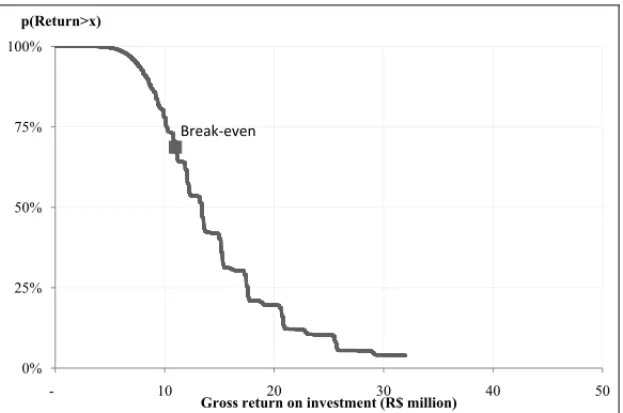
BreakͲeven
Figure 5– Complementary cumulative probability function for gross return on investment.
3 CONCLUSIONS AND FINAL RESULTS
The analysis herein conducted shows that even well-defined problems, such as lottery games, may involve complex phenomena, requiring a careful analysis not to derive misleading insights.
The study evidences that certain kinds of bets have an economical advantage over others, al-lowing for 21 times the coverage for a price only 10 times higher. In spite of this economical advantage, roughly 89% of players choose to play with the cheapest, least efficient ticket, sug-gesting most of them do not fit a rational agent model.
It is also shown that, while 69% of players may be considered to select numbers randomly among the 80 available in the pool, the 31% remaining are twice more likely to select numbers between 1 and 31, here called birthday numbers. As a consequence, the expected number of winners sharply rises when these numbers are drawn, increasing the investment’s risk.
We also showed that the coverage of all the possible drawing’s outcomes is not a trivial problem, requiring a heuristic approach to derive a solution that approaches the optimal. While one could initially estimate R$ 8.6 million would be necessary to cover all the possible results, the algorithm suggests that R$ 11.0 million are, in fact, needed to do so.
The consolidated results, on the other hand, estimates the expected return on investment to be R$ 15.0 million, an upside of 37% over the initial investment, with a 12% chance of doubling the initial investment. On the other hand, there’s also a 31% chance that the return won’t make up for the amount invested and for 71% of these cases the net loss is higher than R$ 1.0 million.
Considering both these points and the enormous operational difficulties for covering all necessary bets, our conclusion is that this unconventional investment opportunity should be recommended only for those with a huge appetite for risk.
Now, before we comment on the results related to the draw of June 24th, 2013, what we will do in the upcoming paragraphs, we find interesting to point out that above conclusions were precisely those that were presented on an early version of this paper that was submitted and accepted for publication on the Proceedings of the Brazilian Symposium on Operations Research (see Castello & Milioni, 2013). Therefore, above conclusions are previous to these results. Let us then present and comment on the final results of the Draw of June 24th, 2013.
As expected, the draw for the 2013 edition of Quina de S˜ao Jo˜ao was held on June, 24th, 2013. There was a considerable coverage from the media and the results can be found in many places, such as http://bit.ly/10I1jFd, for instance. In summary:
• The total prize for winners of the 1st tier (5 correct matches) was R$ 97.5 million.
• The draw numbers were 05, 17, 55, 63 and 67, i.e., two birthday numbers were draw.
• There were 15 winners on the 1sttier and they shared R$ 6.5 million each.
We had predicted:
• A total prize of R$ 97.0 million for the first tier (see Table 5), a difference of only 0.6%
when compared to the real value.
• That two birthday numbers were the most likely situation to occur, with a probability of 36% (see Table 6).
• That, in this case, the expected number of winners of the 1st tier would be 7.7 almost exactly half of what really occurred (again, Table 6).
There is an important point to be considered, here. As it has been seen, our analysis focus only on the frequency that birthday numbers are selected, without taking in consideration specifically which were these numbers. In the draw held on June 24thof 2013, both birthday numbers that were selected, 5 and 17, are very popular among players (see Table 3). Number 5 appears on 2nd place among all numbers, losing only to number 13, while number 17 ranks 12th.
In fact, it is important to mention that above results reinforce the evidence of the hypothesis of player’s bias.
• It is expected thatP had 166 wins on the 2ndtier (see sub-section 2.12). Since there were 2,337 other winners on this tier and each one received a total of R$ 4,398,Pwould expect to receive:
166∗2,337∗4,398
(2,337+166)=R$ 0.68 million.
• Similarly, for the 3rdtier,Pwould expect to have 7,332 wins (see, again, sub-section 2.12), andPwould then expect to receive:
7,332∗130,118∗113
(130,118+7,332)=R$ 0.78 million.
• Therefore, with a single win on the 1sttier,Pwould receive 6.50+0.68+0.78=R$ 7.96 million. In this case, since the investment was R$ 10.98 million (see Table 4), P would have lost R$ 3.02 million.
• It is important to recall, however, that due to imperfections on the covering algorithm (see sub-section 2.7), Phad a probability of 12.5% (1.3%) of winning with two (three) tickets on the 1sttier, cases in whichP’s total prize would be R$ 13.29 (R$ 18.19) million, a gain of R$ 2.31 (7.21) million.
• Thus,P’s expected return would be:
−3.02∗0.862+2.31∗0.125+7.21∗0.013= −R$ 2.22 million.
Therefore, this “unconventional investment opportunity” that showed to be possibly good in 2011 and 2012 would have been catastrophic in 2013, with an expected loss of more than R$ 2 million.
In other words, beating the lottery, after all, is still a matter of luck.
REFERENCES
[1] BURGERA P, GRUNDLINGH¨ WR & VANVUURENJH. 2003a.The Lottery Problem. Available at:
<http://dip.sun.ac.za/∼vuuren/papers/lotery artikel1oud.pdf>. Accessed 21 Oct. 2012.
[2] BURGERAP, GRUNDLINGH¨ WR & VANVUURENJH. 2003b.Two Combinatorial Problems
involv-ing Lottery Schemes: Algorithmic Determination of Solution Sets. Available at:
<http://bit.ly/ZPsC0S>. Accessed 21 Oct. 2012.
[3] CASTELLO J & MILIONIAZ. 2013.Special Lottery Drawings – Analysis of an Unconventional
Investment Opportunity, accepted for presentation and publication on the Proceedings of SBPO 2013
– Brazilian Symposium on Operations Research, September, 16thto 19th, Salvador, BA, Brazil, 2013.
[4] CEF (CAIXAECONOMICAˆ FEDERAL). 2011. Circular Caixa no. 546, de 20 de abril de 2011. Super-intendˆencia Nacional de Loterias. Available at:
<http://www.normasbrasil.com.br/norma/circular-546-2011 11129.html>. Accessed 12 Oct. 2012.
[5] CEF (CAIXAECONOMICAˆ FEDERAL). 2012. Quina. Loterias da Caixa. Available at:
[6] DUPLESSISA. 2010.On two combinatorial optimization problems involving lotteries. Thesis (Mas-ter of Commerce) – Stellenbosch University. Available at: <http://bit.ly/12gDhxG>. Accessed 21 Oct. 2012.
[7] FOG A. 2008. Calculation Methods for Wallenius’ Noncentral Hypergeometric Distribution.
Com-munications in Statistics, Simulation and Computation,37(2): 258–273.
[8] GORDONDM, KUPERBERG G, PATASHNICKO & SPENCERJH. 1995.Asymptotically Optimal
Covering Designs. Available at: <http://www.ccrwest.org/gordon/optimal.pdf>. Acessed 12 Oct.
2012.
[9] GRUNDLICH¨ WR. 2004.Two New Combinatorial Problems involving Dominating Sets for Lottery
Schemes. Tese (Ph.D) Available at:<http://dip.sun.ac.za/∼vuuren/Theses/Grundlingh.pdf>Acessed
12 Oct. 2012.
[10] SIMONSG & JOHNSONNL. 1971. On the convergence of Binomial to Poisson distributions.The
Annals of Mathematical Statistics,42(5): 1735–1736.
[11] THALERRH & ZIEMBAWT. 1988. Parimutuel Betting Markets: Racetracks and Lotteries.Journal