ABSTRACT: Recently, there has been a growing interest in studies concerning ionization sensors for aerospace applications, power generation, and fundamental research. In aerospace research, they have been used for studies of shock and detonation waves. Two key features of these sensors are their short response time, of the order of microseconds, and the fact that they are activated when exposed to high temperature air. In this sense, the present paper describes the development of an ionization sensor to be used in shock tube facilities. The sensor consists of 2 thorium-tungsten electrodes insulated by ceramic, with a stainless steel adapter for proper mounting, as well as 2 copper seal rings. An electrical circuit was also built with 2 main purposes: to provide the electrodes with a sufficient large voltage difference in order to ease ionization of the air and to assure a short time response of the sensor. The tests were carried out in a shock tube with the objective of observing the response of the sensor under stagnation conditions. For that, we chose initial driven pressures of 1.0; 1.2 and 1.5 kgf/cm², with a constant driver pressure equal to 70 kgf/cm². We analyzed the response of the sensor as a function of the initial driven pressure, stagnation temperature, and density. For the studied conditions, the results showed that the mean amplitude of the ionization sensor signal varied from 8.29 to 19.70 mV.
KEYWORDS: Ionization sensors, Shock tubes, Shockwaves.
Experimental Investigation of Ionization Sensors
under Shock Tube Stagnation Conditions
Rafael Augusto Cintra1, Tiago Cavalcanti Rolim2, Bruno Coelho Lima2
INTRODUCTION
Recently, there has been a growing interest in the study of ionization sensors for aerospace applications, energy gener-ation, and fundamental research. In aerospace research, the ionization sensors are generally used in studies on shock and detonation waves (Gupta 2013; Panicker 2008).
In studies of shockwaves, the interest lies on the possibility of using these sensors on shock tube improvement since they can detect high temperature air with an appropriate response time. Shock tubes are used for the simulation of the light conditions of high speed light, for example, atmospheric vehicle reentry. In fact, this kind of facility can create high stagnation temperature and pressure, through a system of tubes illed with diferent pressures. Shockwaves formed by these tubes can achieve very high Mach numbers. In general, the high temperature created by the shockwave allows the dissociation of molecules of N2 and O2 present in the air; however, the temperature is not sufficient to make a direct ionization. Under these circumstances, it is used an ion sensor to create a voltage potential between the 2 electrodes and thus permitting the ionization of the air.
In this work, we show the development of an ionization sensor for shock tube applications. he tests were carried out in the shock tube T1 of the Instituto de Estudos Avançados with the objective of observing the response of the sensor under stagnation conditions to obtain its response in high temperatures.
1.universidade Federal de Itajubá – Instituto de Engenharia Mecânica – Itajubá/MG – Brazil. 2.Departamento de Ciência e Tecnologia Aeroespacial – Instituto de Estudos Avançados – Divisão de Aerotermodinâmica e Hipersônica – São José dos Campos/SP – Brazil.
Author for correspondence: Rafael Augusto Cintra | universidade Federal de Itajubá – Instituto de Engenharia Mecânica | Avenida BPS, 1.303 – Pinheirinho
CEP: 37.500-903 – Caixa Postal: 50 – Itajubá/MG – Brazil | Email: rafaelcintra94@outlook.com
METHODOLOGY
IOnIzATIOn SEnSOR
he ionization sensor is shown in Fig. 1 and it is comprised of 2 electrodes of tungsten-thorium (∅1 mm), mounted diametrically opposite and 1.0 mm apart. his material was chosen due to its capability to support high temperatures with low erosion. In addition to that, the thorium helps the passage of electric current and it also gives more stability and longevity to the sensor. his kind of electrode is widely used in TIG welding. Also, it was used an alumina ceramic material for a good electrical and thermal insulation even at high temperatures. he electrodes were ixed to the ceramic by means of a bicomponent epoxy resin. Two seal rings were used for sealing the sensor. Moreover, it was fabricated with stainless steel clamp nut for adequate seal and an adapter for the sensor to be used in the shock tube.
Figure 2 shows the electrical circuit used for the tests. he choice of the voltage, resistances, and capacitance was based on
the study of Glass and Hall (1959). hese values provide quick response of the sensor, high voltage between the electrodes, and a high-level output signal. In this circuit, the discharge time can be estimated using Eq. 1, and the charge time can be estimated using Eq. 2, as follows:
Clamp nut
Adapter
Seal ring Seal ring
Ceramic Electrodes
Oscilloscope
Electrodes 0.5 nF 10 MΩ
47 kΩ
Switch 300 V
+ –
2,853.45 35.70 2,219.10
5,142.85
Driven DDS Driver
Figure 2. Electrical circuit used with the ionization sensor.
Figure 1. Sectional view of the developed ionization sensor (dimensions in mm).
τ
discharge≈ (47 × 103 Ω)(0.5 × 10⁻⁹ F) = 23.5μsτ
charge≈(10 × 106 Ω)(0.5 × 10⁻⁹ F) = 5mshe electrical circuit presented high level of noise when the switch was on. To circumvent that, the switch could be turned of ater the capacitor charging during the tests. Since the circuit was in open loop, the capacitor did not discharge until ionization of the air.
ShOCK TuBE DESCRIpTIOn
During these tests we used the shock tube T1 (see Fig. 3), which is comprised of 2 reservoirs, one filled with high-pressure gas denominated driver and the other one illed with a low-pressure gas denominated driven. hese 2 reservoirs are separated by a Double Diaphragm Section (DDS), in which 2 diaphragms with known rupture pressures are used to control the test start. his section remains at an intermediate pressure. he entire tube has an internal diameter of 68.00 mm. he driver section has a length of 2,219.10 mm; the driven section, of 2,853.45 mm; and the DDS, of 35.70 mm.
(1)
(2)
Figure 3. Dimensions of shock tube T1 (in mm).
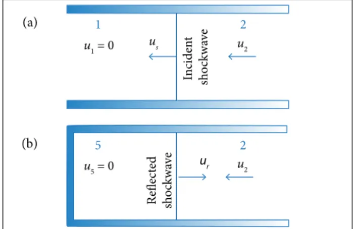
he properties across the incident and relected shock-waves (regions 2 and 5, respectively) are calculated considering chemical equilibrium. The air is modeled as a mixture of gases — N2, O2, NO, N, O, and Ar —, and the inal composition is calculated through Gibbs free energy minimization (details about this procedure are given in Rolim 2013). he thermo-dynamic properties of each species were calculated with the NASA polynomials described by McBride et al. (1993) with updated coeicients given by the thermochemical database of Burcat and Ruscic (2005). he measured values of the incident shockwave speed us, the pressure across the incident shockwave p2 and across the relected shockwave p5 are inputs for the equi-librium calculation, as well as the shock tube initial conditions (pressure p1, temperature T1, density ρ1, and speed of sound a1). he estimated properties across the incident shockwave (which has a Mach number Ms = us/a1) are: the temperature T2, the density ρ2, the low velocity in the laboratory frame u2, the speciic enthalpy h2, and the molar concentration of each species. Likewise, the estimated properties across the relected shockwave are: the temperature T5, the density ρ5, the relected shockwave velocity in the laboratory frame ur, the speciic enthalpy h5, and the molar concentration of each species.
ExpERImEnTAl AppARATuS
he experimental apparatus for the tests is presented in Fig. 5 with the ionization sensor positioned at the end of the driven. hree piezoelectric sensors type PCB 113B26 (PCB Piezotronics 2013) were used to measure the pressure along the tube and to estimate the velocity of incident shockwave by time of light (TOF). he choice of a piezoelectric sensor was due to its fast response required in studies of shockwaves.
he data acquisition system was a Yokogawa oscilloscope type DL750 ScopeCorder with 16 channels, using a signal conditioner type PCB 481 for the pressure sensors. Also, it was used an ultrastable power supply type 70706 to provide 300 V to the circuit. On later tests this power supply was substituted by a power supply fabricated in-house, which has a ripple factor of 1%.
P5 P2.2 P2.1 P2.0
965.39 651.07 337.40 u1 = 0
u5 = 0 u2
u2
In
ciden
t
sho
ck
w
av
e
R
ele
ct
ed
sho
ck
w
av
e
us
u
r
1 2
5 2
(a)
(b)
Figure 4. Shockwave system inside shock tube: (a) Incident shockwave; (b) Relected shockwave.
Ionization sensor
Pressure sensor
Pressure sensor
Electric circuit
Power suply
Oscilloscope Signal conditioner
Figure 6. Position of the pressure sensors along the driven (dimensions in mm).
Figure 5. Schematics of the shock tube tests.
The positions of the pressure sensors along the tunnel are shown in Fig. 6, where P5 is at the end of the driven, and the other sensors are positioned along the driven: P2.2 closer to the end, P2.1 in the middle, and P2.0 in a further position. However, only the pressure signal from the position P2.2 was used for the incident shockwave pressure measurement, and the pressure signal from the position P5 was used for the reflected shockwave pressure measurement. Table 1 shows the technical specifications of the pressure sensors used during the tests.
It was possible to determine the incident shockwave velocity us by measuring the time interval (Δt) between the signals from the sensor in P2.2 position and from the sensor in P5 position. Since the distance between them was known, equal to Δx, one can get the incident shockwave velocity using Eq. 3:
TEST mATRIx
Table 2 shows that the only parameter varied during this investigation was the initial driven pressure. The choice of positioning the sensor at the end of the driven section is justified because the reflected shockwave produces a higher temperature than the incident shockwave, which helps ionization (Anderson 1989).
In Fig. 7, a response of the ionization sensor for the test condition of initial driven pressure of 1.0 kgf/cm
²
is shown. he passage of incident and relected shockwave from the piezoelectric sensors signal was observed. Also, it can be noted that the response of the ionization sensor under stagnation conditions imposed by the shock tube matches with the response of piezoelectric sensors.With the average values presented in Table 3, the sensor signal was analyzed with the variation of the initial driven pressures, stagnation temperature, and stagnation density; the results are shown in Figs. 8, 9, and 10, respectively.
In Fig. 8, it is possible to observe that the signal decreased from 1.81 × 10⁻² to 8.29 × 10⁻³ V (54.2%) when varying the
initial driven pressure from 1.0 kgf/cm² (9.81 × 10⁻² MPa) to
1.5 kgf/cm
²
(1.47 × 10⁻¹MPa) probably due to the decrease instagnation temperature. However, for the cases in which the initial driven pressure varied from 1.0 kgf/cm
²
(9.81 × 10⁻²MPa)Speciication Value
Measurement range 500 lbf/in² Sensitivity 10 mV/(lbf/in²) Maximum pressure 10,000 lbf/in²
Resolution 0.002 lbf/in² Discharge time constant ≥ 50 s
Rise time ≤ 1 µs Output impedance < 100 Ω
Uncertainty ±1.3%
Table 1. General speciication of the sensor PCB113B26 (PCB Piezotronics 2013).
number of valid tests
Initial pressure in driven
[kgf/cm²] Gas in driven
12 1.0 Synthetic air
4 1.2 Synthetic air
5 1.5 Synthetic air
Table 2. Test conditions.
RESULTS AND DISCUSSION
For these tests, the driven was illed with synthetic air at the pressures of 1.0, 1.2, and 1.5 kgf/cm
²
. he driver was illed with helium at the pressure of 70 kgf/cm². he shock tube conditions achieved during these tests are shown in Table 3. Uncertainties were calculated using the methodology presented by the AIAA Standard S-071A-1999, working with a conidence level of 95%.Comparing the Mach number values of experiments with initial driven pressures of 1.0 and 1.2 kgf/cm
²
, it was observed that the average Mach number for 1.2 kgf/cm²
was 2.87, while, for 1.0 kgf/cm²
, 2.82. However, it was expected that the Mach number value at 1.0 kgf/cm²
would be higher than that obtained for 1.2 kgf/cm²
; the authors believe that the variation of the initial driven temperature (T1) contributed to this result.Figure 7. Voltage history for the ionization and pressure sensors with initial driven pressure of 1.0 kgf/cm².
Figure 8. Variation in ionization sensor signal with the initial driven pressure.
0.0 0.2 0.4 0.6 0.8 1.0 1.2 1.4 1.6 1.8 2.0 −2.0
0.0 2.0 4.0 6.0 8.0 10.0 12.0 14.0
Time [ms]
Voltage [V]
Incident Shockwave
Reflected Shockwave
Ionization Sensor
Sensor PCB P5 Sensor PCB P2.2 Sensor PCB P2.1
Ionization Sensor (multiplied by 100)
0.02 0.06 0.10 0.14 0.18 0.000
0.005 0.010 0.015 0.020 0.025 0.030 0.035 0.040 0.045 0.050
Initial driven pressure, p1 [MPa]
Ionization sensor signal [V]
parameter Test condition 1.0 kgf/cm²
Test condition 1.2 kgf/cm²
Test condition
1.5 kgf/cm² unit
p1 9.81 × 10⁴ ± 9.81 × 10³ 1.18 × 10⁵ ± 9.81 × 10³ 1.47 × 10⁵ ± 9.81 × 10³ Pa
T1 293.92 ± 0.81 299.65 ± 2.26 299.55 ± 2.06 K
ρ1 1.16 ± 0.12 1.37 ± 0.11 1.71 ± 0.11 kg/m³
us 970.21 ± 0.12 995.63 ± 30.96 942.05 ± 35.15 m/s
Ms 2.82 ± 0.12 2.87 ± 0.09 2.71 ± 0.10
-a1 343.76 ± 0.12 347.08 ± 1.33 347.02 ± 1.19 m/s
Air properties after incident shockwave
p2 1.07 × 10⁶ ± 7.56 × 10⁴ 1.20 × 10⁶ ± 1.75 × 10⁴ 1.34 × 10⁶ ± 4.35 × 10⁴ Pa
T2 853.27 ± 107.41 795.93 ± 70.97 748.02 ± 61.09 K
ρ2 4.38 ± 0.46 5.23 ± 0.46 6.24 ± 0.47 kg/m³
u2 712.80 ± 32.27 735.43 ± 29.70 683.85 ± 34.02 m/s
h2 5.82 × 10⁵ ± 1.19 × 10⁵ 5.18 × 10⁵ ± 7.79 × 10⁴ 4.66 × 10⁵ ± 6.63 × 10⁴ J/kg
Air composition after incident shockwave
N2 1.18 × 10² ± 1.23 × 101 1.41 × 10² ± 1.24 × 10 1.68 × 10² ± 1.26 × 10 mol/m³
O2 3.18 × 10 ± 3.31 3.80 × 10 ± 3.34 4.53 × 10 ± 3.39 mol/m³
I 1.89 × 10⁻¹¹ ± 8.24 × 10⁻¹¹ 1.66 × 10⁻¹² ± 5.47 × 10⁻¹² 1.63 × 10⁻¹³ ± 5.27 × 10⁻¹³ mol/m³
Ar 1.51 ± 1.58 × 10⁻¹ 1.81 ± 1.59 × 10⁻¹ 2.16 ± 1.62 × 10⁻¹ mol/m³
NO 7.14 × 10⁻⁴ ± 1.10 × 10⁻³ 3.38 × 10⁻⁴ ± 3.86 × 10⁻⁴ 1.66 × 10⁻⁴ ± 1.88 × 10⁻⁴ mol/m³
N 6.43 × 10⁻²⁵ ± 5.36 × 10⁻²⁴ 5.81 × 10⁻²⁷ ± 3.67 × 10⁻²⁶ 6.56 × 10⁻²⁹ ± 4.05 × 10⁻²⁸ mol/m³
Air properties after relected shockwave
p5 4.65 × 10⁶ ± 4.06 × 10⁵ 5.35 × 10⁶ ± 1.19 × 10⁵ 5.73 × 10⁶ ± 1.27 × 10⁵ Pa
T5 1,347.51 ± 235.92 1,239.22 ± 160.96 1,151.39 ± 139.82 K
ρ5 12.0 ± 1.8 15.0 ± 1.9 17.3 ± 2.1 kg/m³
ur 408.33 ± 26.36 392.85 ± 17.71 385.03 ± 16.63 m/s
h5 1.15 × 10⁶ ± 2.83 × 10⁵ 1.03 × 10⁶ ± 1.90 × 10⁵ 9.22 × 10⁵ ± 1.63 × 10⁵ J/kg
Air composition after relected shockwave
N2 3.24 × 10² ± 4.93 × 10 4.05 × 10² ± 5.19 × 10 4.67 × 10² ± 5.58 × 10 mol/m³
O2 8.71 × 10 ± 1.34 × 10 1.09 × 10² ± 1.40 × 10 1.26 × 10² ± 1.50 × 10 mol/m³
O 1.13 × 10⁻⁵ ± 4.30 × 10⁻⁵ 1.82 × 10⁻⁶ ± 5.59 × 10⁻⁶ 3.12 × 10⁻⁷ ± 9.64 × 10⁻⁷ mol/m³
Ar 4.15 ± 6.30 × 10⁻¹ 5.19 ± 6.64 × 10⁻¹ 5.98 ± 7.14 × 10⁻¹ mol/m³
NO 2.21 × 10⁻¹ ± 2.87 × 10⁻¹ 1.36 × 10⁻¹ ±1.39 × 10⁻¹ 7.94 × 10⁻² ±8.28 × 10⁻² mol/m³
N 4.55 × 10⁻¹⁴ ± 3.33 × 10⁻¹³ 1.28 × 10⁻¹⁵ ±7.54 × 10⁻¹⁵ 4.17 × 10⁻¹⁷ ± 2.47 × 10⁻¹⁶ mol/m³
Ionization sensor
Voltage 1.81 × 10⁻² ± 8.99 × 10⁻³ 1.97 × 10⁻² ± 1.31 × 10⁻² 8.29 × 10⁻³ ± 2.75 × 10⁻³ V
Table 3. Estimated properties calculated for initial driven pressures of 1.0; 1.2 and 1.5 kgf/cm². to 1.2 kgf/cm
²
(1.18 × 10⁻¹ MPa), the signal increased from1.81 × 10−2 to 1.97 × 10⁻² V (8.8%).
It was expected that the ionization sensor, when exposed to higher temperatures, would present higher voltage amplitudes, because the high temperature helps the ionization of the
air (Anderson 1989). In Fig. 9, it is shown the variation of sensor signal with the stagnation temperature obtained during the tests. It was observed that the signal increased from 8.29 × 10⁻³ to 1.97 × 10⁻² V (137.6%) with the elevation
however, it decreased from 1.97 × 10⁻² to 1.81 × 10⁻² V (8.1%)
with the elevation of temperature from 1,238.22 to 1,347.51 K, respectively. Similarly, in higher air densities, it was expected that the sensor would present higher voltage amplitudes due to the increase in the total molar concentration. See Table 3 for the air composition after reflected shockwave; note that the molar concentrations of N2, O2, and Ar are much higher than those from other species. In Fig. 10, it is shown the variation of the sensor signal with the stagnation air density, where an increase in the signal was observed when the air density varied from 12.0 to 15.0 kg/m
³
. On the other hand, the signal decreased when density varied from 15.0 to 17.3 kg/m³
. Observing Figs. 9 and 10 one can see a relation type “mirror” between the graphs of temperature and density. This happened because, in this kind of shock tube operation, the temperature decreases when the air density rises, ascan be seen in Fig. 11. Thus, for higher temperatures, there was a drop in the air density, which reduced the voltage amplitude and justified the fact that the point with initial driven pressure of 1.2 kgf/cm
²
presented the highest voltage amplitude.Figure 10. Variation in the ionization sensor signal with stagnation air density.
Figure 9. Variation in the ionization sensor signal with stagnation temperature.
Figure 11. Relationship between the stagnation temperature and the stagnation air density.
5.0 10.0 15.0 20.0 25.0
0.000 0.005 0.010 0.015 0.020 0.025 0.030 0.035 0.040 0.045
Density of the air in stagnation condition, p5 [kg/m³]
Ionization sensor signal [V]
900 1,000 1,100 1,200 1,300 1,400 1,500 1,600 1,700 1,800 0.000
0.005 0.010 0.015 0.020 0.025 0.030 0.035 0.040 0.045 0.050
Temperature of stagnation condition, T5 [K]
Ionization sensor signal [V]
5.0 10.0 15.0 20.0
900 1000 1100 1200 1300 1400 1500 1600
Density of the air in stagnation condition, ρ5 [kg/m³]
Temperature of stagnation
condition,
T5
[K]
CONCLUSIONS
Using the ionization sensor developed in this study, in a shock tube under stagnation conditions, it was possible to observe the behavior of the sensor when exposed to air at high temperatures. he stagnation temperatures varied from 1,151.39 to 1,347.51 K and the stagnation pressures, from 4.65 to 5.73 MPa. Also, it was possible to conclude the following points:
• A fast and consistent response of the ionization sensor signal was obtained.
• In principle, it was expected that the signal of the sensor would be higher when exposed to higher temperatures. However, the air density influenced the sensor signal. In this study, the air density and temperature varied inversely under stagnation conditions, and lower densities would produce fewer ions in the air. Therefore, when the temperature was increased, the air density decreased, and the results of the sensor were a balance between these 2 effects.
AUTHOR’S CONTRIBUTION
Cintra RA and Rolim TC conceived the idea and co-wrote the main text; Cintra RA, Rolim TC, and Lima
BC performed the experiments; Cintra RA prepared the figures and tables; Lima BC helped in the shock tube operation; Rolim TC worked as advisor for Cintra RA.
REFERENCES
Anderson JD (1989) Hypersonic and high temperature gas dynamics. 2nd ed. London: McGraw-Hill.
Burcat A, Ruscic B (2005) Third millennium ideal gas and condensed phase thermochemical database for combustion with updates from active thermochemical tables. ANL-05/20 and TAE 960. Argonne: Argonne National Laboratory and Technion-IIT. doi:10.2172/925269.
Glass II, Hall JG (1959) Handbook of supersonic aerodynamics. Washington, DC: Government Printing Ofice. V. 6, Sec. 18, Shock tubes.’
Gupta NKM (2013) Point measurement of detonation wave propagation using ion gauge (Master’s thesis). Arlington: The university of Texas at Arlington.
McBride BJ, Gordon S, Reno MA (1993) Coeficients for calculating thermodynamic and transport properties of individual species. NASA-TM-4513. Cleveland: NASA.
Panicker PK (2008) The development and testing of pulsed detonation engine ground demonstrators (PhD thesis). Arlington: The university of Texas at Arlington.
PCB Piezotronics (2013) Model 113A26 ICP Pressure Sensor Installation and Operating Manual. Depew: PCB Piezotronics, Inc.