Abstract
This paper investigates the effect of different parameters on stress analysis of infinite orthotropic plates with central polygonal cutout using gray wolf optimization algorithm. The important features of gray wolf algorithm include flexibility, simplicity, short solution time and ability to avoid local optimums. The effective parameters on stress distribution around cutouts include load angle, curvature radius of the corner of the cutout, cutout orientation and fiber angle for orthotropic materials. The used analytical solution is the expansion of Lekhnitskii’s solution method. The effect of the aforementioned parameters on the stress distribution around trian-gular, square, pentagonal and hexagonal cutout is examined. The results showed that these parameters have significant effects on stress distribution around the cutouts and the structural load-bearing capacity will increase without changing the type of material if the parameters are correctly chosen.
Keywords
Orthotropic Plates, Grey Wolf Algorithm, Polygonal Cut-out, Analytical Solution.
Optimum Design of Effective Parameters for Orthotropic
Plates with Polygonal Cut-Out
1 INTRODUCTION
In engineering structures, different types of cut-out are made to satisfy some service requirements. These cut-out result in the strength degradation of structures and may lead to their failure. It is observed that more failures in aircraft structures have happened in fastened joints having high stress concentrations. In order to predict the behaviour of the structures with such cut-out, it is essential to study the effect of cutout geometry and loading conditions on the stress distribution around the cut-out.In fact, cut-out reduce the weight of structures which is desirable for designers. Cut-out are mostly created in plates to reduce the structural weight or to create points of entry and exit. These changes in the plate geometry lead to severe local stresses that is called stress
concentra-Mohammad Jafari a
Mohammad Hossein Bayati Chaleshtari b
a Associate Professor , Department of
Mechanical Engineering, Shahrood University of Technology, Shahrood, Iran. [email protected] b MSc. Student , Department of
Mechanical Engineering, Shahrood University of Technology, Shahrood, Iran. [email protected]
http://dx.doi.org/10.1590/1679-78253437
tion. Hence, knowing the stress concentration factor is crucial in achieving optimal design. The study of the stress distribution in perforated plates was started by Muskhelishvili (1962), Savin (1970) and Lekhnitskii (1969). They used conformal mappings and complex variable method for stress analysis of isotropic and anisotropic plates containing a central cutout. The complex variable method for solving boundary value problems in two- dimensional elasticity was firstly applied by Muskhelishvili (1962) for isotropic plates. Shortly after and applying a similar method, Savin (1970) performed some investigations on infinite isotropic plates with different cut-out and anisotropic plates with only elliptical and circular cut-out. Lekhnitskii (1969) used an analytical solution to investigate the boundary value problems by complex variable method based on Kolosov-Muskhelishvili formulas for anisotropic plates with circular and elliptical cutout. An accumulation of all previous researches on plates containing cut-out was conducted by Sternberg (1958), Neuber (1968) , Peterson (1974) and Pilkey (1997). Theocaris and Petrou (1986) used Schwarz–Christoffel transformation to evaluate the stress concentration factor for an infinite plate with central triangu-lar cut-out. Daoust and Hoa (1991) analyzed the triangutriangu-lar cut-out in infinite isotropic and aniso-tropic plate under uniaxial loading. A part from the equilateral triangle, they investigated other triangular out with different aspect ratios. They also studied the effect of the curvature of cut-out corner on the stress distribution around the triangular cut-cut-out.Asmar and Jabbour (2007) also applied the same theory to investigate the stress distribution around the cut-out in an anisotropic plate with a quasi-square cut-out and subjected to uniaxial loading. But this research studied only the effect of bluntness and cut-out orientation for very special cases. Rezaeepazhand and Jafari (2010) used Lekhnitskii’s theory to study the stress analysis of composite plates with quasi-square cut-out subjected to uniaxial tension. Batista (2011) investigated stress distribution around polygo-nal cut-out with rather complex geometries. He used the expansion of Muskhelishvili’s complex var-iable method and Schwarz-Christoffel mapping function. Ukadgaonker and Rao (1997) presented solutions for stress distribution around triangular cutout with blunt corners in composite plates. Wescott et al. (2004)) investigated the stress analysis of near optimal surface notches in3D plates using two-dimensional (2D) optimal notch shapes. Sharma (2014) presented a general solution to calculate stress distribution around polygonal cut-out in infinite isotropic plates subjected to biaxial loading. He also studied the effect of cutout geometry and the pattern of loading on the stress anal-ysis of perforated plates. Kazberuk et al. (2016) studied stress distribution at sharp and rounded V-notches in quasi-orthotropic plane. Jafari and Ardalani (2016) also studied the stress distribution around several polygonal cut-out in finite isotropic plates. They investigated the effects of cut-out orientation and the bluntness of the polygonal cut-out on the stress concentration.
parame-ters on the optimized mechanical behavior of structures. PSO technique was employed in order to maximize the torsion constant of the structures in this work. Chen et al. (2013) developed a method for optimum designing (based on reliability) of a composite structure based on the combination of PSO and FEA methods. Muc and Gurba (2001) used a combination of genetic algorithm and finite element analysis in optimization of composite structures. Kradinov et al. (2007) showed the applica-tion of genetic algorithm in the optimal design of bolted composite lap joints. Moreover, Suresh et al. (2007) investigated the particle swarm optimization approach for multi-objective composite box-beam design. Kathiravan and Ganguli (2007) showed the application of particle swarm optimization and gradient method in the strength design of composite beams. Jafari and Moussavian (2016) in-vestigated the optimum design of laminated composite plates containing a quasi-square cut-out. They used swarm intelligence algorithms in this research. Mirjalili et al. (2014) have recently tested grey wolf optimizer (GWO) on uni-modal, multi- modal, fixed-dimension multimodal, and compo-site functions. It is efficient in terms of exploration, exploitation, local optimal avoidance, and con-vergence. It has been shown that the grey wolf optimizer algorithm is able to provide very competi-tive results compared to other well-known meta-heuristics. The grey wolf optimizer algorithm has been successfully applied to three classical engineering design problems and real optical engineering (Mirjalili et al. 2014). Song et al. (2014) have successfully applied GWO for solving combined eco-nomic emission dispatch problems. Emary et al. (2015) have used GWO for feature subset selection. Mirjalili (2015) has investigated the effectiveness of GWO in training multi-layer perceptions (MLP). Saremi et al. (2015) proposed the use of evolutionary population dynamics (EPD) in the grey wolf optimizer algorithm to further enhance it is performance. Song et al. (2015) have success-fully applied GWO for parameter estimation in surface waves. In this study, relying on Lekhnitskii’s analytical solution and expanding this solution to the polygonal cut-out in orthotropic plates, the comprehensive stress analysis of perforated orthotropic plates is conducted. In this research design variables are load angle, bluntness, cutout orientation and fiber angle. It is tried to introduce the optimum values of the mentioned parameters for uniaxial tensile loading in order to obtain the min-imum normalized stress. It is worth mentioning that the normalized stress value around the cutout is considered as cost function (C.F.) for grey wolf optimization algorithm. The main goal of this paper is to obtain the optimal design variables which minimize the maximum stress around polygo-nal cutout calculated by apolygo-nalytical method based on complex variable method. The optimal values of these parameters are determined using GWO.
2 THEORY ANALYSIS
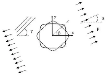
cut-out size is small compared to the size of plate (infinite plate). This investigation is conducted by considering the plane stress state and the absence of body forces. Also, the plate material is in its linear elastic region. Because of the traction-free boundary conditions on the edge of the cut-out, the stresses and at the cutout edge are zero and the circumferential stress is only remaining stress.
Figure 1: Infinite plate with quasi-square cut-out under uniaxial load.
Analytical method used in this study is retrieved from the expansion of analytical solution method by Savin (1961) and Lekhnitskii (1969). In this method, stress function converts to an ana-lytical expression with undetermined coefficients and displacements and stresses could be calculated by stress function being determined. Equilibrium equation will be satisfied by introducing F(x,y) as stress function according to Eq. (1).
2 2
y F x
2 2
x F y
y x
F xy
2
(1)
0 2
) 2
(
2 16 4 3 12 66 24 2 26 43 22 44
4 4
11 x F R y x F R y x F R R y x F R y F R (2)
Eq. (2) is compatibility equation for anisotropic materials where Rijare members of reduced compliancematrix that for plane strain and plane stress states will be according to Eqs. (3) and (4) respectively: 33 2 13 33 11
11 (S S S )/S
R
33 23 13 33 12
12 (S S S S )/ S
R
33 36 13 33 16
16 (S S S S )/S
R
33 2 23 33 22
22 (S S S )/S
R
33 36 23 33 26
26 (S S S S )/S
R
33 2 36 33 66
66 (S S S )/S
R
(3)
R S (i,j=1,2,6) (4)
where S are the transformed compliance matrix components of the lamina and S is determined in terms of compliance matrix components as follows:
S T S T (5)
where [T2] and [T1] are transformation matrix defined as follows:
We have used m=cos and n=sin. is fiber angle. Compliance matrix in terms of engineering constants will be as below:
S
E ν E
ν E ν
E E
ν E ν
E
ν
E E E ν
G
G
(7)
Thus solving 2D planar elasticity problems will lead to presentation and solution of fourth-order differential equation which is expressed by four first-order linear derivative operator as Eq. (8). Lekhnitskii (1969) proved that this characteristic equation associated with orthotropic material generally has four imaginary roots which are mutually conjugated.
0 2
) 2
(
2 16 3 12 66 2 26 22
4
11 R R R R R
R (8)
In curvilinear coordinate systems, the stress components created around the cut-out in two-dimensional region are expressed in terms of the stress functions (z1)and(z2). Lekhnitskii (1969) showed that the stress components around the cut-out in a plate pulled by uniform tension P ap-plied at a considerable distance from the cut-out edge (in theory, it is infinity), at an angle; with respect to the x-axis can be calculated as the Eqs. (9) to (11) (Lekhnitskii, 1969):
( ) ( )
Re 2
cos2 12 z1 22 z2 P
x
(9)
( ) ( )
Re 2
sin2 z1 22 z2
P
y
(10)
( ) ( )
Re 2 sin .
cos 1 z1 2 z2
P
xy
(11)
Where zixiy (i=1,2) and iare the roots of the characteristic equation of anisotropic
Figure 2: Curvilinear coordinates.
In order to calculate the stress components in the polar coordinates system, the Eqs. (12) and (13) are used. According to Figure 2, in these equations is the angle between the positive x-axis and the .
x y
(12)
i
xy x
y i e
i ( 2 ) 2
2
(13)
Stress distribution around the circular cutout was investigated by Savin (1961) using complex variable method. In order to expand their solution to other out, points on boundary of the cut-out with particular shape should be transformed cut-outside the circle with unit radius using a simple mapping function (zi xiy) first, where x and y are obtained from Eqs. (14) and (15):
)) cos( .
(cos
w n
x (14)
)) sin( .
(sin
w n
y (15)
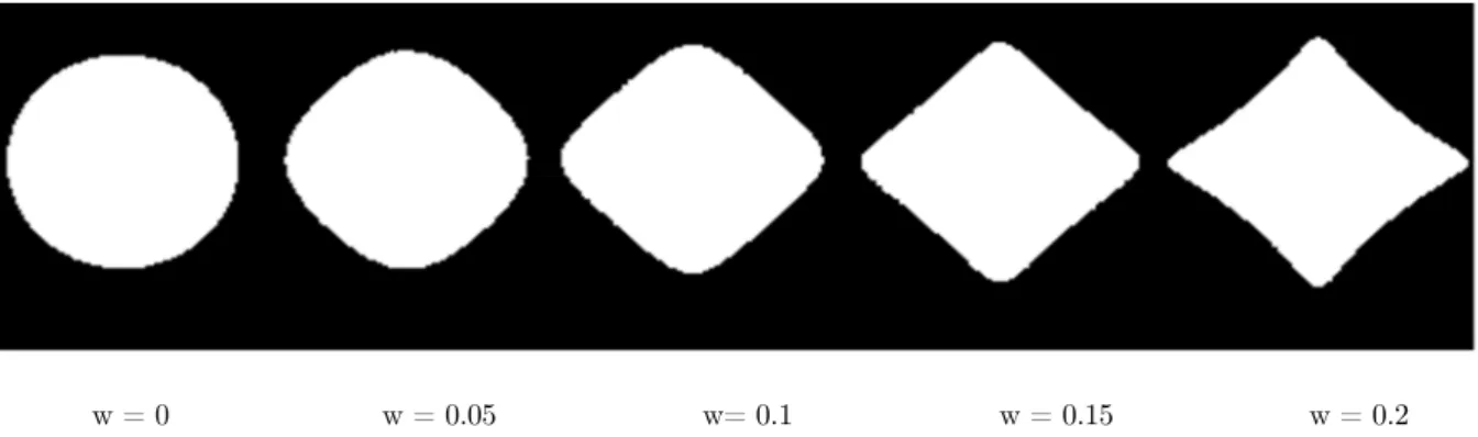
In the above equation, the parameter , which is a positive and real number, controls the size of the cutout. Integer n determines the shape of cut-out. Parameter w is the bluntness factor which changes the radius of curvature at the corner of the cut-out. For example, in above trigonometric equation, for quasi-square cut-out with sides of equal length (equilateral) n should be equal to 3. The conditions 0w<1/n ensure that the cut-out shape does not have loops. Effect of the amount of
w = 0 w = 0.05 w= 0.1 w = 0.15 w = 0.2
Figure 3: The influence of w on the cutout geometry.
n=2 n=3 n=4 n=5 w=0
w=0.3 w=0.15 w=0.1 w=0.08
Figure 4: Effect of w and n on the cutout shape.
3 GREY WOLF OPTIMIZATION (GWO)
Nature is full of social behaviours for performing different tasks. Although the ultimate goal of all individuals and collective behaviours is survival, creatures cooperate and interact in flocks. Wolf packs own one of the most well-organized social interactions for hunting. Grey wolf optimization was proposed by Mirjalili et al. (2014). Mirjalili creates a bio-inspired optimization algorithm, the so called grey wolf optimization (GWO), which has been inspired from the leadership hierarchy and hunting mechanism of grey wolves in nature. He used twenty nine test functions in order to investi-gate the performance of the proposed algorithm in terms of exploration, exploitation, local optima avoidance, and convergence. Then, he proved the grey wolf optimizer results were able to provide highly competitive results compared to well-known heuristics such as PSO, GSA, DE, EP, and ES . In addition, the three main steps of hunting, searching for prey, encircling prey, and attacking prey, are implemented (Mirjalili et al. 2014).
3.1 Mathematical Model
solu-tions are named and respectively. The rest of the candidate solutions are assumed to be . In this paper the hunting mathematical models are provide.
3.1.1 Encircling Prey
A grey wolf can update its position inside the space around the prey in any random location by using Eqs. (16) and (17). The encircling behavior of grey wolves can be represented as : (Mirjalili et al. 2014)
) ( ) (
.X t X t
C
D P (16)
D A t X t X P . ) ( ) 1
( (17)
Where t is the number of iteration, A 2a.r1a and C 2.r2 , are coefficient vectors, XP
is the prey position and X is the gray wolf position. The components of a are linearly decreased from 2 to 0 over the course of iterations. r1 and r2 are random values in [0,1]. The components of a are linearly decreased from 2 to 0 over the course of iterations. Moreover,A is random values in the interval [-a,a] as
, , and .3.1.2 Hunting
In the GWO algorithm, the hunting (optimization) is guided by
, , and. The wolves follow these three wolves.X X C D X X C D X X C D . . . 3 2 1 (18) ) .( ) .( ) .( 3 3 2 2 1 1 D A X X D A X X D A X X (19) 3 ) 1
(t X1 X2 X3
X (20)
X ,X and X
are position vector of ,and respectively. The parameters A and C
for mathematical modeling of approaching to the prey, the value of a is linearly decreased. Thus A is a random value in the interval [-a, a]. When random values of A are in [-1,1] (|A| < 1), GWO forces the wolves to attack towards the prey. The parameter a is decreased from 2 to 0 in order to adaptively emphasize exploration and exploitation, respectively. Candidate solutions tend to diverge from the prey when A 1and converge towards the prey when A 1. Finally, the grey wolf
opti-mization algorithm is terminated by the satisfaction of an end criterion. (Mirjalili et al. 2014)
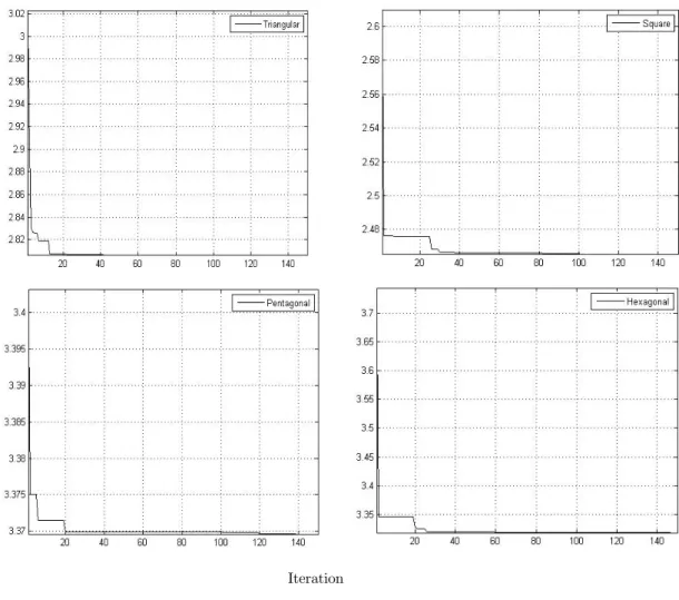
4 TESTING CONVERGENCE GWO
The constraints contain upper and lower boundaries which can be changed based on shape of the cut-out. Figure 5 shows convergence diagrams for GWO algorithm for Glass/Epoxy plate containing cut-out with various shapes in one of the optimum conditions (w=0.05, =30). The ratio of the maximum stress created around cutout to the applied stress is considered as cost function.
Cost F
unc
tion(C.F.)
Iteration
In Figure 5, in addition to viewing the convergence for the intended condition, it can be seen that GWO algorithm always tries to search local optimum value that finding the absolute optimum value in a suitable time. Also, the duration of solving the GWO algorithm after several runs, it turned out that GWO algorithm is capable of finding the absolute optimum value in a short time.
5 RESULTS
Many parameters affect the stress distribution around cut-out in orthotropic plates. The correct choice of these parameters is an important role in the design of these plates. In this study, an at-tempt has been made to obtain the optimal values of different parameters to achieve the lowest stress concentration for various cut-out. Mechanical properties used in this study are presented in Table 1.
Material E1(GPa) E2(GPa) G12 (GPa) Glass/Epoxy (CE
9000) 47.4 16.2 7 0.26
Graphite/Epoxy
(T300/5208) 181 10.3 7.17 0.28
Carbon/Epoxy
(GY-70/934) 294 6.4 4.9 0.23
Table 1: Materials properties of perforated plate (Rezaeepazhand and Jafari, 2015).
5.1 Quasi-triangular cut-out
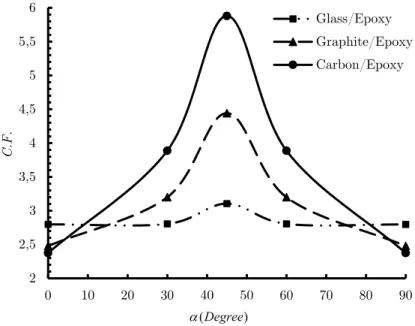
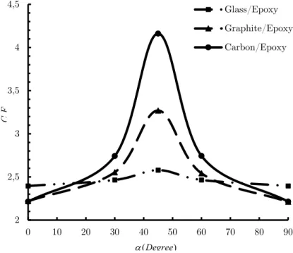
At first for a particular value of w, the optimal values of design variables such as load angle, rota-tion angle of cut-out and fiber angle are calculated. For this purpose, Figure 6 shows the effects of load angle on the value of the cost function by considering fiber angles and cut-out orientation sim-ultaneously as design variables for the discussed three types of orthotropic materials in quasi-triangular cutout with w=0.05. Values of fiber angle and cut-out orientation in this case, are opti-mum values obtained by GWO algorithm. According to the Figure 6, for all three materials, the maximum value of the cost function occurs at loading angle of 45°, and Carbon/Epoxy material has the highest value of stress amongst the three others. For five different load angles, the optimal val-ues of design variables and corresponding cost function inw=0.05 are shown in Table 2. Moreover, Figure 7 shows the variation of the minimum normalized stress with fiber angle for w = 0.05. In fact in this figure for each fiber angle, the value of minimum normalized stress is obtained for optimum values of load angle and rotation angle.
Figure 6: Variations of the cost function in terms of load angle for quasi- triangular cut-out (w=0.05).
) (Degree
Figure 7: Variations of the cost function in terms of fiber angle for quasi- triangular cut-out (w=0.05). 2
2,5 3 3,5 4 4,5 5 5,5 6
0 10 20 30 40 50 60 70 80 90
Glass/Epoxy Graphite/Epoxy Carbon/Epoxy
C.
F.
2 2,5 3 3,5 4 4,5 5 5,5 6 6,5
0 10 20 30 40 50 60 70 80 90
C.
F
.
Glass/Epoxy
Graphite/Epoxy
Carbon/Epoxy )
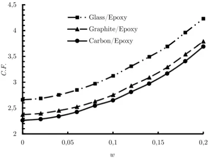
Figure 8: Variations of the cost function in terms of w for quasi-triangular cut-out.
Figure 8 shows the variation of the cost function with respect to w. in this case, the design var-iables are load angle, fiber angle and rotation angle and the cost function has been calculated in the optimal values of them. As illustrated in this figure, for all used materials, the cost function de-creases when the value of bluntness parameters (w) decreases. Therefore, the minimum cost func-tion occurs in w =0 which is equivalent to a circular cut-out. Finally, the optimal values of all pa-rameters listed in Table 5.
Carbon/Epoxy Graphite/Epoxy Glass/Epoxy C.F. C.F. C.F. 2.3747 0 90 0 2.4788 0 90 0 2.7982 180 64.8640 0 3.8870 62.1 90 30 3.1997 177 90 30 2.8048 153.4997 90 30 5.8798 80.71 0 45 4.4415 7.577 90 45 3.1044 119.1598 90 45 3.8867 148.3 90 60 3.1993 92.996 0 60 2.8051 176.4992 0 60 2.3747 150.41 0 90 2.4788 89.95 0.134 90 2.7980 28.7296 27.4888 90
Table 2: Optimal values of different parameters for triangular cut-out in various load angles (w=0.05).
Carbon/Epoxy Graphite/Epoxy Glass/Epoxy C.F. C.F. C.F. 2.3747 29.99 90 0 2.4788 89.95 89.96 0 2.7992 180 61.804 0 3.8843 58.30 90 30 3.1991 63.015 90 30 2.8059 26.50 90 30 5.8791 4.775 90 45 4.4421 22.566 0 45 3.1049 135.83 90 45 3.8864 31.722 0 60 3.1997 87 0 60 2.8058 63.518 0 60 2.3746 180 0 90 2.4788 60.01 0 90 2.8007 90.52 28.522 90
Table 3: Optimal values of different parameters for triangular cut-out in various fiber angles (w=0.05). 2 2,5 3 3,5 4 4,5
0 0,05 0,1 0,15 0,2
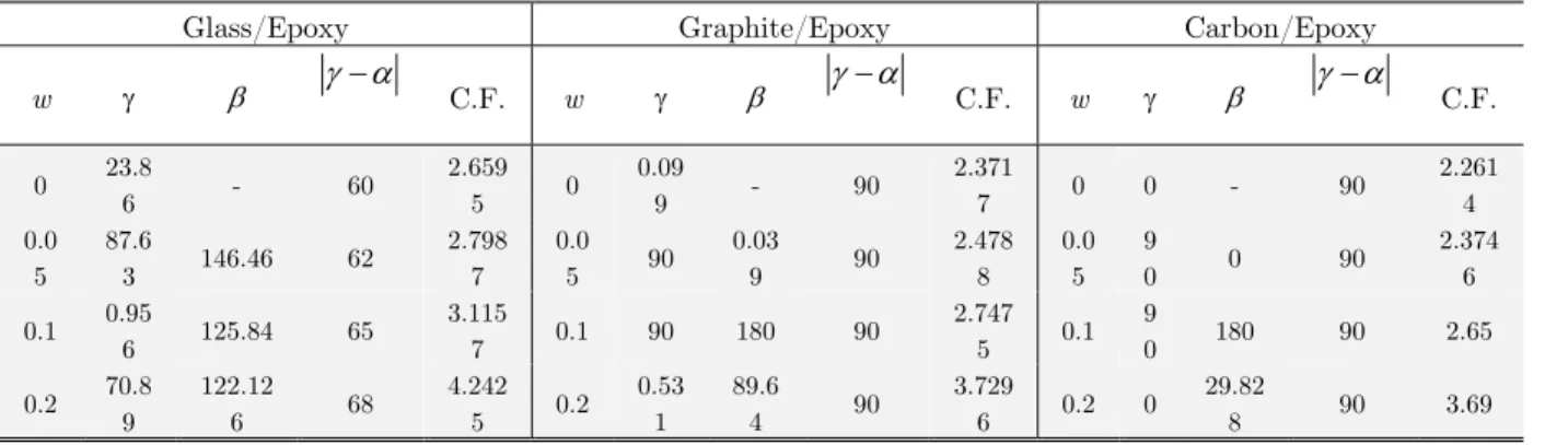
Carbon/Epoxy Graphite/Epoxy Glass/Epoxy C.F. w C.F. w C.F. w 2.261 4 90 - 0 0 2.371 7 90 - 0.09 9 0 2.659 5 60 - 23.8 6 0 2.374 6 90 0 9 0 0.0 5 2.478 8 90 0.03 9 90 0.0 5 2.798 7 62 146.46 87.6 3 0.0 5 2.65 90 180 9 0 0.1 2.747 5 90 180 90 0.1 3.115 7 65 125.84 0.95 6 0.1 3.69 90 29.82 8 0 0.2 3.729 6 90 89.6 4 0.53 1 0.2 4.242 5 68 122.12 6 70.8 9 0.2
Table 4: Optimal values of different parameters for triangular cut-out for different w.
C.F. w Material 2.6595 60 - 18.3 0 Glass/Epoxy 2.3717 90 - 88.21 0 Graphite/Epoxy 2.2614 90 - 0.001 0 Carbon/Epoxy
Table 5: Overall optimum results of triangular cut-out.
5.2 Quasi-Square Cut-Out
Figure 9 shows the effects of loading angle on the value of the cost function by considering fiber angle and cut-out orientation simultaneously as design variables for the discussed three types of anisotropic materials with w=0.05. The values of fiber angle and cut-out orientation in this case, are optimum values obtained by GWO algorithm. According to the Figure 9, for Carbon/Epoxy material, the maximum value of the cost function occurs at loading angle of 45° and it has the high-est value of stress amongst the three others materials. Tables 6 show the optimum values of fiber angle, rotation angle and minimum normalized stress corresponding to each loading angle in
Figure 9: Variations of the cost function in terms of load angle for quasi- square cut-out (w=0.05).
Figure 10: Variations of the cost function in terms of fiber angle for quasi-square cut-out (w=0.05). 2
2,5 3 3,5 4 4,5
0 10 20 30 40 50 60 70 80 90
Glass/Epoxy
Graphite/Epoxy
Carbon/Epoxy
2 2,5 3 3,5 4 4,5
0 10 20 30 40 50 60 70 80 90
Glass/Epoxy Graphite/Epoxy Carbon/Epoxy
γ(Degree)
C.
F
.
) (Degree
Figure 11: Variations of the cost function in terms of w for quasi-square cut-out.
Table 9 shows overall optimum results for the anisotropic material. This results optimization process take place for all parameters such as; fiber angle (γ), load angle (), rotation angle () and cutout curvature (w).
Carbon/Epoxy Graphite/Epoxy Glass/Epoxy C.F. C.F. C.F. 2.214 45 90 0 2.2192 44.9973 90 0 2.3956 44.7 69.4123 0 2.7423 19.2805 90 30 2.5542 9.20499 90 30 2.4650 79.113 90 30 4.1613 59.9335 0 45 3.2691 63.6778 0 45 2.5786 12.456 90 45 2.744 70.01 0 60 2.542 80.7989 0 60 2.4651 77.531 0 60 2.214 44.5932 0 90 2.2191 44.9671 0 90 2.3956 45.375 0 90
Table 6: Optimal values of different parameters for square cut-out in various load angles (w=0.05).
Carbon/Epoxy Graphite/Epoxy Glass/Epoxy C.F. C.F. C.F. 2.2141 44.99 90 0 2.2193 44.66 89.78 0 2.3958 29.39 73.8445 0 2.7427 10.70 90 30 2.554 20.801 90 30 2.4651 40.64 90 30 4.1615 14.687 90 45 3.2690 18.51 90 45 2.5589 58.16 0.6380 45 2.7428 79.29 0 60 2.5539 69.19 0 60 2.4651 49.34 0 60 2.2141 45 0 90 2.2196 46.02 0.663 90 2.3956 60.58 16.1255 90
Table 7: Optimal values of different parameters for square cut-out in various fiber angles (w=0.05). 2 2,2 2,4 2,6 2,8 3 3,2 3,4 3,6 3,8
0 0,02 0,04 0,06 0,08 0,1 0,12 0,14
w Glass/Epoxy Graphite/Epoxy Carbon/Epoxy
Carbon/Epoxy Graphite/Epoxy
Glass/Epoxy
C.F.
w C.F.
w C.F.
w
2.2614 90
- 0 0 2.3717 90
- 0 0 2.6595 60
- 85.2 0
2.2141 90
44.96 0
0.05 2.2191 90
44.99 90 0.05 2.3956 73
44.73 16.2 0.05
2.9664 68
0.706 90
0.1 2.6887 90
44.99 90 0.1 2.7037 90
45.10 90
0.1
5.3198 64
18.73 26.17 0.2 5.3587 90
63.34 90 0.2 4.8959 90
46.13 90
0.2
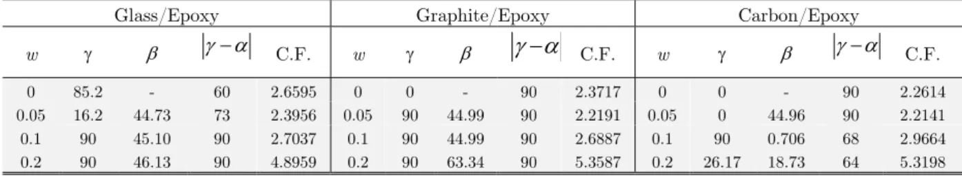
Table 8: Optimal values of different parameters for square cut-out for different w.
C.F.
w Material
2.3918 45
90 0
0.0323241 Glass/Epoxy
2.1691 45
0 90 0.0323241
Graphite/Epoxy
2.1081 45
90 0
0.0260045 Carbon/Epoxy
Table 9: Overall optimum results of square cut-out.
5.3 Pentagonal Cut-Out
Figure 12 shows the effects of loading angle on the values of the cost function by considering fiber angle and cutout orientation simultaneously as design variables for the discussed three types of or-thotropic materials in pentagonal cut-out with w = 0.05. As shown in this figure, for all used mate-rials, the maximum normalized stress occurs at load angle of 45 degrees and Carbon/Epoxy materi-al has the highest vmateri-alue of stress amongst the three others. Moreover, minimum cost function hap-pens at 0 or 90 degrees. For five different load angles, the optimal values of design variables and corresponding cost function in w=0.05 are shown in Table 10.
Figure 12: Variations of the cost function in terms of load angle for pentagonal cut-out (w = 0.05).
Figure 13: Variations of the cost function in terms of fiber angle for pentagonal cut-out (w = 0.05). 2,5
3,5 4,5 5,5 6,5 7,5
0 10 20 30 40 50 60 70 80 90
Glass/Epoxy Graphite/Epoxy Carbon/Epoxy
2 3 4 5 6 7 8
0 10 20 30 40 50 60 70 80 90
Glass/Epoxy
Graphite/Epoxy
Carbon/Epoxy
C.
F.
) (Degree
C.F.
Figure 14: Variations of the cost function in terms of w for pentagonal cut-out. Carbon/Epoxy Graphite/Epoxy Glass/Epoxy C.F. C.F. C.F. 2.796 36 90 0 2.9251 180 90 0 3.3389 144.42 64.80 0 4.778 102.267 90 30 3.9122 133.324 90 30 3.3697 35.494 90 30 7.175 1.666 90 45 5.373 34.7828 90 45 3.7153 25.531 90 45 4.779 59.7031 0 60 3.912 136.721 0.23 60 3.3699 90.622 0 60 2.796 125.912 0.07 90 2.925 125.403 1.15 90 3.3387 17.463 25.38 90
Table 10: Optimal values of different parameters for pentagonal cut-out in various load angles (w=0.05).
Carbon/Epoxy Graphite/Epoxy Glass/Epoxy C.F. C.F. C.F. 2.7966 53.98 90 0 2.9246 53.99 90 0 3.3404 100.09 64.581 0 4.7837 89.81 90 30 3.9139 130.63 90 30 3.3698 156.49 90 30 7.1067 61.65 90 45 5.355 64.37 90 45 3.7168 73.325 90 45 4.7797 72.24 0 60 3.9118 103.33 0 60 3.3695 41.434 0 60 2.797 180 0 90 2.9251 0 0.001 90 3.3394 25.815 25.309 90
Table 11: Optimal values of different parameters for pentagonal cut-out in various fiber angles (w=0.05). 2 2,5 3 3,5 4 4,5 5
0 0,02 0,04 0,06 0,08 0,1
w Glass/Epoxy
Graphite/Epoxy
Carbon/Epoxy
Carbon/Epoxy Graphite/Epoxy Glass/Epoxy C.F. w C.F. w C.F. w 2.2614 90 - 90 0 2.3717 90 - 0 0 2.6595 60 - 78.519 0 2.796 90 88.71 1.278 0.05 2.9251 90 125.62 0.611 0.05 3.3392 66 0.99 8.251 0.05 3.8251 90 125.77 0.114 0.1 4.0161 90 53.84 0.082 0.1 4.6647 66 130.9 90 0.1 6.1308 90 13.66 2.305 0.15 6.2186 90 18.06 0.033 0.15 7.3227 66 74.61 69.69 0.15
Table 12: Optimal values of different parameters for pentagonal cut-out for different w.
C.F. w Material 2.6595 60 - 59.483 0 Glass/Epoxy 2.3717 90 - 90 0 Graphite/Epoxy 2.2614 90 - 0 0 Carbon/Epoxy
Table 13: Overall optimum results of pentagonal cu-tout.
5.4 Hexagonal Cut-Out
For hexagonal cut-out with w = 0.05, the cost function changes with load angle is shown in Figure 15. As shown in this figure, for all used materials, the maximum and minimum values of the cost function occur at load angle of 45 degrees and 0 or 90 degrees, respectively. Table 14 shows the optimum values of fiber angle, rotation angle and minimum normalized stress corresponding to each loading angle in w = 0.05. Moreover, Figure 16 shows the changes of the cost function for various fiber angles in plates with hexagonal cut-out (w=0.05). Load angle and cut-out orientation consid-ered as design variables. As seen in this figure, the maximum of the normalized stress occurs at fiber angle of 45 degrees. Between all used materials and for fiber angle in the range of 20-70 degrees, the highest normalized stress takes place for Carbon/Epoxy material. For different fiber angles, Table 15 shows the optimal values of load angle and rotation angle and corresponding normalized stress. Also, the optimal values of design variables such as rotation angle, load angle and fiber angle in different values of w are shown in Table 16. Figure 17 shows the changes of the cost function with respect to w. In this case, design variables are load angle, fiber angle and rotation angle. According to this figure, the optimal value of w is not zero. Finally, the optimal values of all effective parame-ters are present in Table 17.
Carbon/Epoxy Graphite/Epoxy Glass/Epoxy C.F. C.F. C.F. 2.8495 60.01 90 0 2.8995 0.017 90 0 3.1743 0 90 0 3.6408 4.598 90 30 3.3799 57.88 90 30 3.3184 36.05 90 30 4.87 75.08 90 45 4.098 79.28 0 45 3.3926 31.01 0 45 3.6386 25.47 0.037 60 3.3788 32.16 0 60 3.3221 53.75 0.273 60 2.8495 90 0.001 90 2.8995 90 0.023 90 3.1739 90 0.089 90
Figure 15: Variations of the cost function in terms of load angle for pentagonal cut-out (w = 0.05).
Figure 16: Variations of the cost function in terms of fiber angle for hexagonal cut-out (w = 0.05). ,
, , , , , ,
Glass/Epo Graphite/Epo Carbon/Epo
2,5 3 3,5 4 4,5 5
0 10 20 30 40 50 60 70 80 90
Glass/Epoxy
Graphite/Epoxy
Carbon/Epoxy
C.F.
) (Degree
) (Degree
Figure 17: Variations of the cost function in terms of w for hexagonal cut-out. Carbon/Epoxy Graphite/Epoxy Glass/Epoxy C.F. C.F. C.F. 2.8495 90 90 0 2.8996 90 89.99 0 3.1739 19.99 79.2944 0 3.6359 55.47 90 30 3.3788 62.16 90 30 3.3177 23.94 90 30 4.8699 30.09 0 45 4.09 25.64 0 45 3.3925 13.96 0 45 3.6447 34.66 0.04 60 3.3829 27.98 0.085 60 3.3184 6.063 0.0036 60 2.8495 59.98 0 90 2.8996 0.441 0.247 90 3.1739 0 0.0086 90
Table 15. Optimal values of different parameters for hexagonal cut-out in various fiber angles (w=0.05). Carbon/Epoxy Graphite/Epoxy Glass/Epoxy C.F. w C.F. w C.F. w 2.2614 90 -90 0 2.3717 90 - 0 0 2.6595 60 -76.043 0 2.8495 90 0.072 90 0.05 2.8995 90 0.025 90 0.05 3.1739 90 0.01 90 0.05 4.6234 90 29.85 0 0.1 4.5897 90 0.06 90 0.1 5.0534 79 78.99 0.06 0.1 9.7817 90 27.86 90 0.15 10.0553 90 51.63 90 0.15 10.6522 79 66.42 85.626 0.15
Table 16: Optimal values of different parameters for hexagonal cu-tout for different w.
C.F. w Material 2.5606 60 89.3265 25.2487 0.0096 Glass/Epoxy 2.2855 90 29.6097 0 0.00817 Graphite/Epoxy 2.1983 90 90 0 0.006302 Carbon/Epoxy
Table 17: Overall optimum results of hexagonal cut-out. 2 2,5 3 3,5 4 4,5 5 5,5
0 0,02 0,04 0,06 0,08 0,1
With the increasing number of cutout sides, the obtained results will be close to results of a cir-cular cut-out. The results of the previous sections suggest that the optimal values of the cost func-tion for all cut-out with odd number of sides are always more than the corresponding value of a circular cut-out while all cut-out with an even number of sides are more efficient than a circular cut-out.
6 CONCLUSIONS
In this study, using gray wolf optimization algorithm (GWO), optimum parameters affecting nor-malize stress around polygonal cutout in orthotropic plates were determined. Design variables in this study are loading angle, cut-out orientation, fiber angle and bluntness. The grey wolf optimiza-tion algorithm is another form of metaheuristic algorithms based on swarm intelligence (SI) that draws inspiration from the social leadership hierarchy and hunting behavior of grey wolves in na-ture. Results demonstrated that GWO creates a good balance between exploration and exploitation that results in high local optimal avoidance and a suitable convergence. Moreover, the cost function considered in this paper was obtained based on Lekhnitskii’s solution technique which was just for circular and elliptical cut-out and was generalized to polygonal cut-out using conformal mapping and complex variable method. The results also showed that the cut-out bluntness is not the only parameter affecting the reduction of stress concentration, but also the cut-out orientation, and suit-able load angle and fiber angle play a major role in the reduction of stress that with choosing the optimum values of these parameters in a specific curvature, stress concentration can be reduced significantly. The optimal values of normalized stress for all cut-out with an odd number of sides were always more than the corresponding value of a circular cut-out while, all cut-out with an even number of sides were more efficient than circular cut-out. Among of all cut-out shapes, quasi-square cut-out has the lowest possible normalized stress.
References
Asmar G. H., Jabbour T.G. (2007). Stress analysis of anisotropic plates containing rectangular holes. International Journal of Mechanics and Solids 2(1):59-84.
Barbosa, I. C. J., Loja, M. A. R. (2014). Design of a laminated composite multi-cell structure subjected to torsion. 29th Congress of the International Council of Aeronautical Sciences ICAS 2014: 1–8.
Batista, M. (2011). On the stress concentration around a cutout in an infinite plate subject to a uniform load at infinity. International Journal of Mechanical Sciences 53(4): 254–261.
Chen, J., Tang, Y., Ge, R., An, Q., Guo, X. (2013). Reliability design optimization of composite structures based on PSO together with FEA. Chinese Journal of Aeronautics 26(2): 343–349.
Daoust, J., Hoa, S. V. (1991). An analytical solution for anisotropic plates containing triangular cut-out. Composite Structures 19(2):107-130.
Emary, E., Zawbaa, H.M., Grosan, C., Hassenian, A.E. (2015). Feature subset selection approach by Gray Wolf Optimizer. Advances in Intelligent Systems and Computing 334: 1–13.
Jafari, M., Ardalani, E. (2016). Stress concentration in finite metallic plates with regular cut-out. International Jour-nal of Mechanical Sciences 106: 220-230.
Kazberuk, A., Savruk, M. P., Chornenkyi, A. B. (2016). Stress distribution at sharp and rounded V-notches in quasi-orthotropic plane. International Journal of Solids and Structures 85-86: 134–143.
Kradinov, V., Madenci, E., Ambur, D. R. (2007). Application of genetic algorithm for optimum design of bolted composite lap joints. Composite Structures 77(2): 148–159.
Lekhnitskiy, S. G. (1969). Anisotropic Plates, Gordon and Breach Science, New York.
Mirjalili, S. (2015). How effective is the Grey Wolf Optimizer in training multi-layer perceptrons. Applied Intelligence 43:150-161.
Mirjalili, S., Mirjalili, S.M. Lewis, A. (2014). Grey Wolf Optimizer. Advances in Engineering Software, 69: 46–61. Moussavian, H., Jafari, M. (2016) Optimum design of laminated composite plates containing a quasi-square cutout. Structural and Multidisciplinary Optimization. doi:10.1007/s00158-016-1481-7.
Muc, A., Gurba, W. (2001). Genetic algorithm and finite element analysis in optimization of composite structures. Composite Structures 54:275-281.
Muskhelishvili, N. I. (1953). Some basic problems of mathematical theory of elasticity, Netherlands: oordhooff, Gro-ningen, Holland 56-104.
Neuber, H. (1968). On the effect of stress concentration in cosserat continua, Springer, verlag Berlin Heidelberg. Peterson, R.E. (1974). Stress concentration factors, John Wiley and Sons Inc, New York.
Pilkey, W. D. (1997). Peterson’s stress concentration factors, John Wiley and Sons Inc, Second Edition, New York. Rezaeepazhand, J., Jafari, M. (2010). Stress analysis of composite plates with Quasi-square cut out subjected to uniaxial tension. Journal of Reinforced Plastics and Composites 29:2015–2026.
Saremi, S., Mirjalili, S.Z., Mirjalili, S.M.(2015). Evolutionary population dynamics and grey wolf optimizer. Neural Computing and Applications 26:1257–1263.
Savin, G. N. (1961). Stress concentration around cut-out, Pergamon Press, NewYork.
Sharma, D. S. (2014). Moment distribution around polygonal cut-out in infinite plate. International Journal of Me-chanical Sciences 78(1):177–182.
Song, H.M., Sulaiman, M.H. Mohamed, M.R.(2014). Anapplication of grey wolf optimizer for solving combined eco-nomic emission dispatch problems. International Review on Modelling and Simulations, 2: 838–844 .
Song, X., Tang, L., Zhao, S., Zhang, X., Li, L., Huang, J., Cai, W. (2015). Grey Wolf Optimizer for parameter esti-mation in surface waves. Soil Dynamics and Earthquake Engineering 75: 147–157.
Sternberg, E. (1958). Couple-stresses and singular stress concentrations in elastic solids, Springer, verlag Berlin. Suresh, S., Sujit, P. B., Rao, A. K. (2007). Particle swarm optimization approach for multi-objective composite box-beam design. Composite Structures 81(4):598–605.
Theocaris, P. S., Petrou, L. (1986). Stress distributions and intensities at corners of equilateral triangular cut-out. International Journal of Fracture 31(4): 271–289.
Ukadgaonker, V. G., Rao, D. K. N. (1999). Stress distribution around triangular cut-out in anisotropic plates. Com-posite Structures 45(3): 171–183.
Vigdergauz, S. (2001). The effective properties of a perforated elastic plate Numerical optimization by genetic algo-rithm. International Journal of Solids and Structures 38:8593–8616.