www.atmos-chem-phys.net/13/3661/2013/ doi:10.5194/acp-13-3661-2013
© Author(s) 2013. CC Attribution 3.0 License.
Atmospheric
Chemistry
and Physics
Geoscientiic
Geoscientiic
Geoscientiic
Geoscientiic
Top-down estimate of surface flux in the Los Angeles Basin using
a mesoscale inverse modeling technique: assessing anthropogenic
emissions of CO, NO
x
and CO
2
and their impacts
J. Brioude1,2, W. M. Angevine1,2, R. Ahmadov1,2, S.-W. Kim1,2, S. Evan2, S. A. McKeen1,2, E.-Y. Hsie1,2, G. J. Frost1,2, J. A. Neuman1,2, I. B. Pollack1,2, J. Peischl1,2, T. B. Ryerson2, J. Holloway1,2, S. S. Brown2, J. B. Nowak1,2,
J. M. Roberts1,2, S. C. Wofsy3, G. W. Santoni3, T. Oda4,5, and M. Trainer2
1Cooperative Institute for Research in Environmental Sciences, University of Colorado, Boulder, Colorado, USA 2Chemical Sciences Division, Earth System Research Laboratory, National Oceanic and Atmospheric Administration, Boulder, Colorado, USA
3Harvard University, School of Engineering and Applied Sciences and Department of Earth and Planetary Sciences, Cambridge, Massachusetts, USA
4Cooperative Institute for Research in Atmospheres, Colorado State University, Fort Collins, Colorado, USA 5Global Monitoring Division, Earth System Research Laboratory, National Oceanic and Atmosphere Administration, Boulder, Colorado, USA
Correspondence to:J. Brioude ([email protected])
Received: 22 November 2012 – Published in Atmos. Chem. Phys. Discuss.: 6 December 2012 Revised: 11 March 2013 – Accepted: 12 March 2013 – Published: 2 April 2013
Abstract.We present top-down estimates of anthropogenic CO, NOxand CO2 surface fluxes at mesoscale using a La-grangian model in combination with three different WRF model configurations, driven by data from aircraft flights dur-ing the CALNEX campaign in southern California in May– June 2010. The US EPA National Emission Inventory 2005 (NEI 2005) was the prior in the CO and NOxinversion cal-culations. The flux ratio inversion method, based on linear relationships between chemical species, was used to calcu-late the CO2inventory without prior knowledge of CO2 sur-face fluxes. The inversion was applied to each flight to esti-mate the variability of single-flight-based flux estiesti-mates. In Los Angeles (LA) County, the uncertainties on CO and NOx fluxes were 10 % and 15 %, respectively. Compared with NEI 2005, the CO posterior emissions were lower by 43 % in LA County and by 37 % in the South Coast Air Basin (SoCAB). NOxposterior emissions were lower by 32 % in LA County and by 27 % in the SoCAB. NOx posterior emissions were 40 % lower on weekends relative to weekdays. The CO2 pos-terior estimates were 183 Tg yr−1in SoCAB. A flight during ITCT (Intercontinental Transport and Chemical Transforma-tion) in 2002 was used to estimate emissions in the LA Basin
1 Introduction
The Los Angeles (LA) Basin, a large urban area with emis-sions from mobile sources, industry and agriculture, is a chal-lenging region for chemical-transport models. Regulations controlling emissions of ozone precursors have helped in re-ducing the average ozone concentration in this region. Previ-ous studies have shown reductions in CO and NOxemission factors from mobile sources (Bishop and Stedman, 2008; Dallman and Harley, 2010) and from point sources (Frost et al., 2006) in the US. Furthermore, a recent study has shown a steady decrease in emission of VOCs over the past decades in the South Coast Air Basin (SoCAB; Warneke et al., 2012). However, those large reductions over time result in substan-tial uncertainties in surface emission estimates of ozone pre-cursors based on bottom-up inventories from previous years and impact the accuracy of air quality forecasts. A recent study has also shown that a substantial weekend effect exists in the LA Basin, such that large reductions in NOxemissions on weekends relative to weekdays result in higher weekend ozone production efficiencies (Pollack et al., 2012). These observations provide opportunities to assess the ability of emission inventories to capture interannual and day-of-week variability in the Basin’s emissions and the impacts of these emissions changes on air quality.
Beside ozone precursors, urban areas are significant sources of greenhouse gases (Gurney et al., 2009). Duren and Miller (2012) reported that 70 % of fossil-fuel CO2emissions worldwide were located in urban areas. They stressed that ac-curate emission estimates based on top-down approaches for the largest cities in the world are needed to better assess the carbon emission trends. Aircraft measurements can be used to estimate CO2 emissions in urban areas when combined with an inverse modeling approach (Brioude et al., 2012a). Brioude et al. (2012a) have showed that the Houston, Texas, (USA) area has one of the largest concentrations of anthro-pogenic CO2 sources globally due to a combination of ur-ban and industrial emissions. The State of California has re-cently adopted a cap-and-trade program to control emissions of greenhouse gases. Accurate estimates of anthropogenic greenhouse gas surface fluxes will be necessary to determine if emissions changes mandated under this program have had the desired effects.
In May and June 2010, the NOAA (National Oceanic and Atmospheric Administration) organized and led the CalNex intensive field campaign that took place in the Los Ange-les Basin and Central Valley (Ryerson et al., 2013). These regions are challenging for mesoscale models due to a va-riety of phenomena influencing pollution transport, such as “Catalina” eddies off the coast of southern California, land– sea breezes, and upslope transport from complex terrain sur-rounding the basin (Angevine et al., 2012). In this paper, we use in situ aircraft measurements from the NOAA P-3 along with the Weather Research and Forecasting (WRF) mesoscale model in an application of an inversion technique
to estimate and improve the CO and NOy surface fluxes from the US Environmental Protection Agency’s (EPA’s) Na-tional Emission Inventory (NEI) for the reporting year 2005. The NEI provides the basis for national air quality regula-tory (http://www.epa.gov/scram001/guidanceindex.htm) and forecast modeling (http://www.weather.gov/aq/). The NEI is a “bottom-up” inventory that relies predominantly on emis-sion calculations based on fuel consumption, source activity, and emission factors for most sectors of the US economy.
In this paper, we used NOAA P-3 aircraft observations from the CalNex 2010 campaign and three different WRF configurations at mesoscale as input to the FLEXPART La-grangian particle dispersion model to evaluate and improve a version of the NEI 2005 emission inventory (see Sect. 2 for details). Typically, aircraft observations are temporally sparse compared to measurements from surface stations. However, aircraft are capable of measuring, during a sin-gle flight, several pollutants upwind and downwind of sur-face sources (industries, urban areas). Furthermore, aircraft can sample pollutants at different distances downwind of a source, allowing evaluations of model emissions, chem-istry, and dynamics. In contrast to satellites, most P-3 mea-surements in CalNex provide a spatial resolution of 100 m horizontally and 10 m vertically, with well-understood mea-surement uncertainties typically on the order of 10–15 %.
We optimized surface emission fluxes from 3 chemical species that are predominantly emitted by anthropogenic sources: CO, NOx and CO2. We calculated CO, NOx and CO2best estimates for 2010 using 6 P-3 flights in May and June 2010 during the CalNex campaign. To address the ques-tion of interannual emission trends, we employed aircraft measurements from a NOAA P-3 flight during the ITCT ((In-tercontinental Transport and Chemical Transformation) 2002 campaign over the LA Basin to calculate CO, NOxand CO2 surface emissions in May 2002 (see Sect. 2 for details). We used three configurations of the WRF mesoscale model and FLEXPART to simulate the transport between the surface sources and the location of the aircraft measurements. The NEI 2005 inventory was used as the prior estimate for CO and NOxemissions in the inversion method. The CO2 pos-terior estimates were calculated from the flux ratio inversion method (Brioude et al., 2012a), which allows the calculation of a posterior at mesoscale without a prior estimate. Section 2 presents the details of the methodology. The results are pre-sented in Sect. 3, and the interpretations of these results are discussed in Sect. 4. Conclusions and further implications of this work are presented in Sect. 5.
2 Method
2.1 Observations
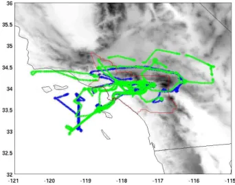
and CalNex 2010 field intensives. In our inverse modeling analysis, we used one flight in 2002 (13 May) and six flights in 2010, 3 during weekdays and 3 during weekends. All of these were flights dedicated to characterizing daytime emis-sions and chemistry in the Los Angeles Basin area. Figure 1 represents the tracks of the 2010 flights. Vertical mixing at night is very uncertain in models and measurements, and therefore nighttime data were not used in this study. Only the observations in the boundary layer were used in the in-version.
CO on the research aircraft was measured once per second using vacuum ultraviolet resonance fluorescence (Holloway et al., 2000) with an uncertainty of±(1 ppbv+0.05×CO). NO and NO2were measured by ozone chemiluminescence (Ryerson et al., 2000; Pollack et al., 2011). CO2was mea-sured by a wavelength-scanned cavity ring-down absorption instrument with an uncertainty of±0.13 ppmv (Peischl et al., 2012). All those species were measured once per second. For the flight on 8 May, we used measurements of CO2 from a Quantum Cascade Laser Direct Absorption Spectrom-eter (QCLS) (Kort et al., 2011). The QCLS measurements have precisions of±0.02 ppm with accuracies of±0.1 ppm (Wofsy et al., 2011). HNO3was measured once per second by chemical ionization mass spectrometry (CIMS) with a precision of 0.012 ppbv and an uncertainty of 15 % (Neu-man et al., 2012). PAN was measured once every 2 s by CIMS, with an uncertainty of±(20 %+0.005 ppbv). NO−3 was recorded every 10 seconds by a aerosol mass spectrome-ter (AMS) with an uncertainty of 30 % (Bahreini et al., 2009). The P-3 data from CalNex are publicly available at www.esrl. noaa.gov/csd/tropchem/2010calnex/P3/DataDownload.
We focus on NOy rather than NOx in our analysis be-cause NOy includes all reactive nitrogen compounds. NOx (=NO+NO2) can be converted to other NOy components (e.g., HNO3 and organic nitrates) on timescales of a few hours, while NOyis a considered as a conserved tracer un-der the conditions of this dataset (see details below). The as-sumption that NOy is a conservative tracer is strengthened by confining the analysis to daytime, when heterogeneous N2O5hydrolysis is unimportant. NOywas calculated as the sum NOy=(NOx+PAN+HNO3+NO−3). NOx, PAN and HNO3were averaged every 10 s. NO−3, when available, was converted into ppbv and added to the sum. NO−3 could ac-count for up to 40 % of NOy on the eastern part of the basin. On the 14 May 2012 flight, the NO and NO2 were measured by cavity ring-down spectroscopy (CRDS; Wagner et al., 2011). When simultaneously available, the CRDS NO and NO2data are in quantitative agreement with the chemi-luminescence measurements. For the 2002 flight, NOywas measured by ozone chemiluminescence with an uncertainty of±(0.20 ppbv+0.12×NOy) (Ryerson et al., 2000). NO−3 measurements were not used for the 2002 flight. NO−3 was measured in the 2002 flight every 4 min (Orsini et al., 2003), which was inadequate for this analysis. NO−3 contributed to
Fig. 1. Map of the domain showing the flight tracks from the 3 weekday flights (blue) and 3 weekend flights (green) of the NOAA P-3 aircraft during CalNex used in this study. The red region refers to the South Coast Air Basin (SoCAB) area.
7.5 % of the NOy concentration in 2010. Therefore, NOy concentrations in 2002 might be underestimated by 7.5 %. Since the chemical transformations are not considered in our analysis, changes in NOyare interpreted as changes in NOx emissions (see Pollack et al., 2012 for a more detailed expla-nation).
No rain clouds were associated with the six CalNex flights or the flight during ITCT used in this analysis. The measure-ments in the LA Basin (Fig. 1) were not far from the sur-face sources, hence secondary production of CO can be ne-glected. The Los Angeles Basin area does not have a large number of power plants, and therefore the effect of NOyloss within power plant plumes (Brock et al., 2003; Neuman et al., 2004) should be small for emission estimates in Los Angeles County or the SoCAB. (Note that conversion to particulate nitrate is taken into account by inclusion of NO−3 in the cal-culated NOy.) We think that the uncertainty on the surface flux in the posterior from assuming NOyis a passive tracer is lower than other sources of uncertainties from WRF (in-cluding wind speed, wind direction, and planetary boundary layer height) or FLEXPART (from linear interpolations or turbulent mixing). We assume that CO and NOyare passive tracers throughout the paper, regardless of the position of the measurements relative to the sources.
2.2 Prior emission inventory
The 4×4 km EPA NEI 2005 weekday inventory version 2 (US Environmental Protection Agency, 2010) is used as the prior emission estimate for the optimization of CO and NOy surface emission inventories. We used the same NEI 2005 inventory as in Brioude et al. (2011). Emissions from point sources, mobile sources on-road and off-road and sur-face areas were processed following EPA recommendations. For details on the mobile emissions models and data source used, see Brioude et al. (2011).
In the paper, the CO and NOyposterior estimates are com-pared with the NEI 2005 (the prior) and CARB 2008 (http: //www.arb.ca.gov/app/emsinv/fcemssumcat2009.php) emis-sion estimates at county level. The anthropogenic CO2 pos-terior estimates are compared to the Vulcan inventory (http:// vulcan.project.asu.edu/, Gurney et al., 2009) at county level, and the statewide 2009 CARB greenhouse gas inventory ap-portioned by population at county level (Peischl et al., 2012). Along with NEI 2005 and the posterior estimates, a CARB 2010 projection is also used in the WRF-Chem v3.4 Eulerian model simulations of tropospheric chemistry (see Sect. 4 for details). Replacing CARB 2008 with the CARB 2010 pro-jection results in only a 9 % reduction in CO and NOx emis-sions. Since CARB 2010 is a projection, it involves addi-tional uncertainties compared with CARB 2008. To down-scale the CARB 2010 projection to a 4×4 km inventory, the NEI-05 emission inventory is modified for 6 counties in southern California according to the CARB (California Air Resources Board) 2010 projected emissions available at http://www.arb.ca.gov/app/emsinv/fcemssumcat2009.php. We refer to this product as the gridded CARB inventory. To conduct chemistry runs with WRF-Chem, VOC emissions in Los Angeles were estimated using the CO posterior es-timates from the inversion used this study and from observed CO-VOC emission ratios (Borbon et al., 2013). See the Sup-plement for further details.
2.3 Modeling
To simulate the atmospheric transport at mesoscale, we used an approach similar to Brioude et al. (2011) for estimat-ing anthropogenic fluxes from the Houston area. Briefly, we used different configurations from a mesoscale meteorolog-ical model as input to the FLEXPART Lagrangian model to estimate uncertainties from the meteorological modeling. See Brioude et al. (2011) for a detailed discussion on uncer-tainties.
Meteorological data were simulated by three different Weather Research and Forecasting (WRF) mesoscale re-search model configurations that were used to drive the FLEXPART Lagrangian particle dispersion model. The dif-ferences between these three models allow us to esti-mate the model uncertainty in the inversion process. Each WRF run was initialized and provided boundary
condi-tions from the ERA-Interim reanalysis (Dee et al., 2011), which has a horizontal resolution of roughly 0.7◦×0.7◦.
The soil was initialized with the ERA-Interim soil tem-perature and moisture fields without spin-up. Sea sur-face temperature input was the US Navy GODAE high-resolution SST (see http://www.usgodae.org/ftp/outgoing/ fnmoc/models/ghrsst/docs/ghrsst doc.txt), updated every six hours and interpolated between updates. The RRTMG short-wave and longshort-wave radiation schemes were used.
The first meteorological configuration used was WRF ver-sion 3.3 with nested grids of 36, 12, and 4 km spacing with two-way nesting. Angevine et al. (2012) evaluated the per-formance of several WRF configurations against a variety of data. The FLEXPART runs reported here used their configu-ration EM4N, and used the Noah land surface model (Chen and Dudhia, 2001; Chen et al., 2011) with MODIS land use and land cover data and the single-layer urban canopy model. The Grell–Devenyi cumulus scheme was used for the outer domain only. The vertical grid had 60 levels, with 19 be-low 1 km and the be-lowest level at approximately 16 m. Run EM4N used the Mellor–Yamada–Janjic planetary boundary layer (PBL) and surface layer options (Janjic, 2002; Suselj and Sood, 2010).
The second configuration used WRF-Chem version 3.1 with nested grids at 36, 20, and 4 km spacing with 60 ver-tical levels. The Noah land surface model was used along with the single-layer urban canopy model. Urban areas were remapped using the National Land Cover Data set (NLCD) 2001. The YSU boundary layer scheme was used. See Lee et al. (2011) for further details.
The third configuration was the WRF-Chem version 3.4 model with two nested grids at 12 km and 4 km horizon-tal spacing with 41 vertical levels. In these runs the Mellor– Yamada–Nakanishi–Niino Level 2.5 (MYNN) PBL bound-ary layer scheme was used. The Noah land surface model with an urban canopy model and the RRTMG longwave and shortwave radiation schemes were used. To parameter-ize deep or unresolved convection, the Grell 3-dimensional (3-D) scheme was activated in the outer domain only. The detailed description of all WRF3.4 parameterizations can be found in http://www.mmm.ucar.edu/wrf/users/docs/user guide V3/contents.html.
Table 1.Linear correlations between observed and simulated time series of CO mixing ratio for the weekday P-3 flights during CalNex 2010 using 3 transport models and the NEI 2005 inventory or the CO posterior in 2010. Results of the ensemble of the 3 transport models are also shown.
Linear correlation using NEI 2005
CO observation
WRF-Chem 3.1
WRF-Chem 3.4
WRF 3.3 Ensemble
CO observation 1
WRF-Chem 3.1 0.69 1
WRF-Chem 3.4 0.69 0.77 1
WRF 3.3 0.74 0.77 0.80 1
Ensemble 0.76 0.93 0.92 0.91 1
Linear correlation using CO posterior
CO observation
WRF-Chem 3.1
WRF-Chem 3.4
WRF 3.3 Ensemble
CO observation 1
WRF-Chem 3.1 0.81 1
WRF-Chem 3.4 0.79 0.83 1
WRF 3.3 0.81 0.82 0.83 1
Ensemble 0.86 0.95 0.94 0.93 1
over 24 h to focus on the local transport within the basin and for computation reasons. The influence of previous day trans-port is ignored but could increase the uncertainty in the flux estimates. Tests performed with 48 h trajectories showed that the surface fluxes based on 24 h trajectories might be over-estimated by 6 % in the LA Basin (not shown). The FLEX-PART output had a resolution of 8×8 km. The output con-sists of a residence time in the surface layer weighted by the atmospheric density. When this output is combined with a surface flux emission inventory, one can calculate a mixing ratio for each set of trajectories along the aircraft flight track. In this way, FLEXPART linearizes the transport processes between the surface and the aircraft, so that an adjoint model of WRF-Chem is unnecessary to apply an inverse modeling technique.
In the paper, we use the term “transport model” for a com-bination of one of the WRF mesoscale model runs and FLEXPART. We assume that each transport model is inde-pendent. Table 1 presents the linear correlation between the CO measurements on weekdays in 2010 and each simula-tion using the NEI 2005 prior inventory. The correlasimula-tion co-efficients between the various simulations of CO time series are not much larger than the coefficients for the correlations between any given model and the observed CO time series, which confirms that each model simulation can be considered as independent in a sense that there is no correlation bias. The CO time series in the ensemble of the three transport models has the highest correlation coefficient when compared to the measurements.
Table 2 shows the average absolute error between the ob-served CO and simulated CO mixing ratios using the NEI 2005 prior inventory for the three weekday six P-3 flights considered in this study. Figure 2 presents the distribution of points compared with the observations. Each transport
model has an error of about 180 ppb of CO on average, for an average measured above-background CO concentration of 86 ppb. As shown by Angevine et al. (2012), these large bi-ases cannot be explained by uncertainties in the transport models, and instead they most likely reflect an overestima-tion of surface emissions in the NEI inventory. Therefore, an inversion method is needed to optimize the NEI prior esti-mates.
2.4 Inverse modeling
We applied an inverse modeling approach on a domain that covers the SoCAB and the mountains surrounding the basin. We employed the same method as Brioude et al. (2011, 2012a). In this section we summarize the techniques used. See Brioude et al. (2011, 2012a) for further details.
For each flight, a chemical background level was estimated and subtracted from the measured mixing ratios. We defined the chemical background of CO and NOyas the lowest mix-ing ratio found in the atmospheric boundary layer upwind (offshore measurements included) of the Los Angeles Basin. The chemical background value of CO2was estimated from the vertical distribution of CO2mixing ratios obtained during each flight near the top of the boundary layer, over the basin. We treated CO, NOyand CO2as passive tracers (see Sect. 2.1 for further details). Only the observations in the boundary layer were used in this study.
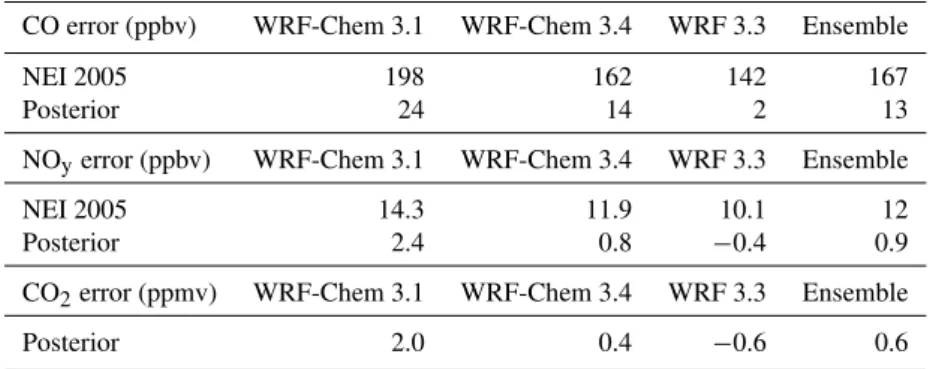
Table 2.Average errors in CO, NOyand CO2mixing ratios for the weekday CalNex P-3 flights using the 3 different WRF configurations
or the ensemble and using NEI 2005 or posterior estimates. The average measured concentration above background was 86 ppb for CO, 10.6 ppb for NOy, and 9.6 ppm for CO2.
CO error (ppbv) WRF-Chem 3.1 WRF-Chem 3.4 WRF 3.3 Ensemble
NEI 2005 198 162 142 167
Posterior 24 14 2 13
NOyerror (ppbv) WRF-Chem 3.1 WRF-Chem 3.4 WRF 3.3 Ensemble
NEI 2005 14.3 11.9 10.1 12
Posterior 2.4 0.8 −0.4 0.9
CO2error (ppmv) WRF-Chem 3.1 WRF-Chem 3.4 WRF 3.3 Ensemble
Posterior 2.0 0.4 −0.6 0.6
Fig. 2.Scatter plots of observed and simulated CO mixing ratio above background using the NEI 2005 inventory (red dots) or the CO posterior from the inversion (black dots) based on the ensemble of the three transport models for the three flights during weekdays. The dash line represents the one-to-one line shown for reference.
function in a 4-dimensional (4-D=3 spatial dimensions plus time) least squares method following Brioude et al. (2011). The advantage of using a log-normal cost function is that no negative fluxes are found in the posterior. This approach avoids the drawbacks of techniques used to prevent negative fluxes that have no particular meteorological basis (e.g. Stohl et al., 2009).
We used a Bayesian least squares method to invert the ob-served concentrations and determine the surface fluxes. The covariance matrix of the observations includes uncertainties from the measurements and the background definition for each flight and is assumed to be diagonal. The observation error is assumed to be uncorrelated. The covariance matri-ces of the observation and prior estimate are not perfectly known, and therefore uncertainties in the posterior can arise from the assumptions made about those covariance
matri-ces. To overcome this issue, we used the L-shape criterion method to balance the errors in both covariance matrices to obtain a posterior estimate with the smallest sensitivity to the error in either the observation or prior covariance matrices (Brioude et al., 2011; Henze et al., 2009). The uncertainty in the prior covariance matrix is assumed to be 100 % be-fore applying the L-curve criterion. The grid cells used in the inversion are restricted to those with a significant anthro-pogenic emission in the NEI 2005 prior to reduce the size of the matrices involved. Those with negligible emissions (the white grid cells in Figs. 3–5) are not used in the anal-ysis. This restriction prevents the inversion from inferring new surface sources and could result in significant uncertain-ties in the posterior. However, no fires were observed during the flights used in the inversion, and the grid cells used in the inversion cover a large area of the basin. Therefore, re-moving grid cells with negligible anthropogenic emissions should not significantly impact the posterior flux estimates. We included 4 time steps in the 4-D inversion: one time step representing nighttime emissions between 01:00–13:00 UTC (local time, LT, during CalNex was UTC−7 h), a time step between 13:00 and 17:00 UTC that includes the morning rush hour, a time step between 17:00 and 21:00 UTC to represent midday conditions, and a time step between 21:00 UTC to 01:00 UTC that includes the evening rush hour. These time steps were chosen based on the overall weekday diurnal cy-cle in the NEI for the SoCAB and the temporal distribution of the aircraft observations during CalNex, which occurred between 16:00 UTC and 01:00 UTC. The values reported in Sect. 3 are the averages for the two time steps between 17:00 UTC and 01:00 UTC where we have the strongest con-fidence in the transport models and therefore in the inversion. However, the differences found between the posterior and the NEI prior vary by only a few percent when the time step be-tween 13:00–17:00 UTC is also used in the comparisons.
least squares method would give a posterior CO2 flux es-timate with a highly uncertain spatial distribution. There-fore, we instead employed the flux ratio inversion method (Brioude et al., 2012a), which takes advantage of the linear relationships between CO2and the tracers CO and NOythat are co-emitted with CO2. We further used our best estimates of CO and NOyposterior surface fluxes to infer a CO2 pos-terior within an inversion framework.
For each posterior inventory, a mean value and a standard deviation is given for the SoCAB and LA County emission estimates. The standard deviation includes the variability in the surface flux, the uncertainty of the method, and the un-certainty in the transport models. The unun-certainty from the Lagrangian model cannot be assessed with this approach, but this uncertainty is small compared to the uncertainties in the meteorological fields. Brioude et al. (2012b) showed that there is no mass conservation problem with the WRF-FLEXPART model combination within the domain of inter-est.
In Sect. 3.4, the surface flux estimates from the single flight in 2002 are compared to the posteriors in 2010. The CO and NOyinversions in 2010 were tested by using either all the flights combined (3 flights during weekdays or 3 flights during weekends) or by performing inversions on each flight individually. Interestingly, the average fluxes found in 2010 with a combination of flights or with a single flight are iden-tical at the county level. Instead of combining all the flights in 2010, we calculated the posterior estimates from each in-dividual flight to estimate the uncertainty of the emissions reported here from single-flight-based inversions. Therefore, the uncertainty of using a single flight in 2002 can be as-sessed more accurately. Furthermore, the estimates in 2010 were averaged using the 3 flights during weekdays and week-ends to evaluate any weekend effect in the surface emissions. The uncertainty in the posterior estimates from using a single flight is discussed in detail in Sect. 4.
3 Results
3.1 CO
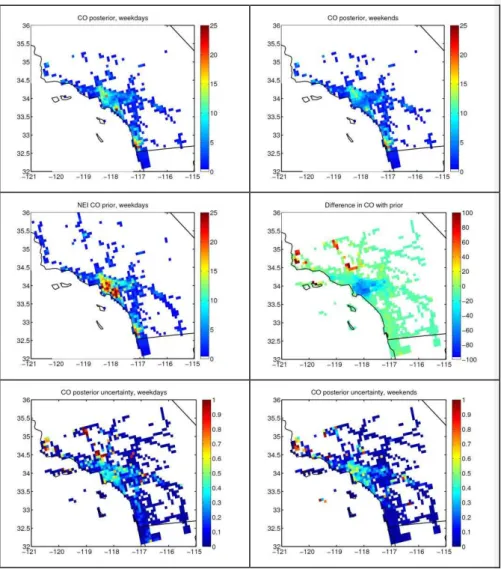
The daytime EPA NEI CO inventory (defined as the average values from 17:00 UTC to 01:00 UTC, or 10:00–18:00 LT) is characterized by large emissions in the urban area that includes Los Angeles and Orange Counties (Fig. 3) and by on-road emissions, mainly from highways. Lower emissions fluxes are found over the suburbs east of Los Angeles.
The posterior inventories, averaged for the inversions with the three models, show the same emission pattern as the prior (Fig. 3), but with large reductions in CO emissions from the Los Angeles/Irvine urban areas. Each grid cell in the poste-rior has an uncertainty of about 20 to 40 % in the Los An-geles County area. The uncertainty (1-σ standard deviation) is estimated from the ensemble of realizations of the three
models with a random term in the prior and with a variabil-ity of 10 % for each flight (a total of 90 realizations). The uncertainty of these average fluxes includes the uncertainty from the meteorological models and the inversion method, and also the natural variability of the surface sources. There-fore, these uncertainty estimates should be considered as un-certainties on the mean, but not necessarily as unun-certainties due to the method. The uncertainty is lower along the coast and is higher in complex terrain, where it is more difficult for the inverse modeling technique to converge to a single solu-tion due to the transport uncertainties associated with large terrain changes within a single grid cell or a few adjacent cells (Brioude et al., 2012b).
The percentage differences in CO emissions between the prior and posterior during weekdays (Fig. 3) clearly show that the emissions reduction is limited to the urban area. Large increases are also found along Interstate Highway 5 in the mountains north of Los Angeles, but these grid cells are associated with large uncertainties (100 %) and relatively small fluxes.
Any single grid cell has a numerical uncertainty from the model that can be reduced by averaging the surface fluxes over several grid cells. We report in Table 3 the daytime emissions in the prior and posteriors from two different re-gions: LA County and the SoCAB. These regions are associ-ated with mostly relatively flat terrain areas, and should not suffer from biases due to complex terrain that could occur in FLEXPART (Brioude et al., 2012b). The daytime average CO posterior estimates can be converted to daily average es-timates by multiplying the daytime eses-timates by 0.7, based on the hourly variation in NEI 2005.
Compared to the NEI, the daytime CO emissions from LA County during weekdays are reduced by 43 %, with an uncertainty of 6 %. The SoCAB emissions are reduced by 37 %±10 %. Figure 3 also shows the posterior estimates for weekend flights. The CO emission pattern on weekends looks similar to that on weekdays, CO emissions during weekends are reduced by 18 % in LA County and by 15 % in SoCAB compared to weekday emissions. This weekday– weekend modulation is in agreement with a recent study of CalNex observations (Pollack et al., 2012) based on in situ measurements from the NOAA P-3 aircraft and surface site measurements that found a weekday CO reduction of 9 % on average.
Fig. 3.Daytime average surface flux of CO during weekdays (10−9kg s−1m−2, top left) and weekends (top right); daytime average surface flux of CO in the NEI 2005 inventory (middle left); difference between the weekday posterior and NEI prior CO estimates (middle right); fractional uncertainties in the posterior during weekdays (bottom left) and weekends (bottom right).
The difference in total emissions between LA County and SoCAB is an estimate of how the emission distribution in the basin varies between the NEI, CARB and posterior invento-ries. In NEI, the CO emissions in SoCAB are higher by 57 % compared to LA County. In our posterior CO inventory, So-CAB emissions are higher by 74 % than LA County, showing that the emissions outside LA County are relatively larger in the posterior than in the NEI prior. In other words, the inverse method modified the spatial distribution of the CO surface fluxes compared to the prior. The SoCAB-LA County CO difference in the CARB inventory is 68 %, in better agree-ment with the distribution in the posterior compared with the NEI.
3.2 NOy
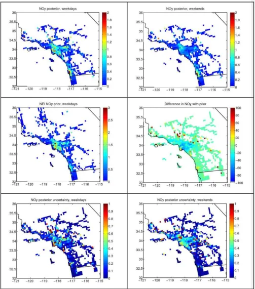
Fig. 4.Same as Fig. 3, but for NOyemissions.
the three models) are reduced by 32 %±10 % in Los Ange-les County (Table 3), while emissions in the SoCAB region are reduced by 27 %±15 % during weekdays. The posterior-prior difference in NOyemissions in the port is even larger, with a reduction of a factor of 5. Kim et al. (2011) have shown that probable sources of this NOydiscrepancy are as-sociated with overestimates of the port NOxemissions from commercial marine vessels within the NEI 2005 area inven-tory and overestimates of the industrial point source NOx emissions in the NEI 2005 point source inventory.
Figure 4 also presents the daytime posterior NOyestimate during weekends. The emissions are lower in the Los Ange-les urban area and surroundings than during weekdays. The difference between weekdays and weekends is 43 % in LA County and 40 % in the SoCAB area. Those results agree with Pollack et al. (2012), who found a reduction of 34 % to 46 % based on in situ measurements.
The emission estimates in the NOyposterior estimate are in better agreement with CARB 2008 than with NEI 2005 for LA County, with a reduction of 6 % during weekdays and 17 % during weekends compared to CARB emissions. These reductions are within the uncertainty range of our inversion calculations. In the SoCAB region, the differences between CARB 2008 and the posterior NOyare+7 % during week-days and−2 % during weekends, also within the uncertainty range. In contrast, total NOyemissions in the SoCAB region are higher than LA County by 57 % in NEI 2005, 48 % in CARB 2008 and 69 % in the posterior. This result indicates that emissions are larger outside LA County in the posterior than in either of the bottom-up inventories.
Table 3.Total daytime emissions (average from 17:00 UTC to 01:00 UTC, 10:00–18:00 LT) of CO, NOyand CO2in Los Angeles County
and the South Coast Air Basin (SoCAB) during weeday and weekend from NEI 2005 inventory, CARB 2008 inventory and the posteriors in 2010 from the inversion technique applied in this study. Based on NEI 2005 and Vulcan 2002 diurnal profiles, the daytime posterior estimates of CO, NOyand CO2can be multiplied by 0.7, 0.78 and 0.78, respectively, to convert them into daily average estimates, based on
NEI diurnal profile.
Daytime emission CO NOy CO2
(kg s−1) in 2010 Weekday Weekend Weekday Weekend Weekday Weekend
LA County NEI 2005 69 69 9.0 9.0 N/A N/A
Posterior 39±2.2 32±6.4 6.1±0.6 3.5±0.9 4590±290 4930±670 CARB 2008 34.1 39.7 6.5 4.2 N/A N/A
SoCAB NEI 2005 108 108 14.1 14.1 N/A N/A
Posterior 68±6.6 58±7.6 10.3±1.5 6.1±1.4 7440±390 8200±700 CARB 2008 57.3 68.0 9.6 6.2 N/A N/A
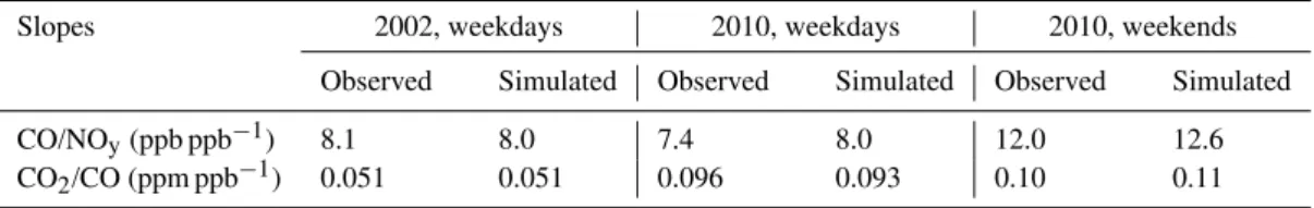
Table 4.Observed and simulated slopes between CO, NOyand CO2mixing ratios in 2002 and 2010 during weekdays and weekends in the
LA Basin.
Slopes 2002, weekdays 2010, weekdays 2010, weekends
Observed Simulated Observed Simulated Observed Simulated
CO/NOy(ppb ppb−1) 8.1 8.0 7.4 8.0 12.0 12.6
CO2/CO (ppm ppb−1) 0.051 0.051 0.096 0.093 0.10 0.11
simulated slope is 10.4 ppb ppb−1using the NEI 2005. Dur-ing weekends, the observed slope is 12 ppb ppb−1while the simulated slope is 12.6 ppb ppb−1. The simulated slope is 10.3 ppb ppb−1using the NEI 2005. These results show that the simulated slopes using the posterior CO and NOy esti-mates are closer to the observed slopes than using NEI 2005. Based on these differences between observed and simulated slopes, we estimate that a bias of about 10 % exists in our CO or NOyflux estimates.
3.3 CO2
As explained in Sect. 2, CO2 posterior estimates are based on the flux ratio inversion method, which allows estimates of CO2(or any species) at mesoscale without using a prior estimate. The linear relationships of CO2 with co-emitted species like CO and NOy, and their surface flux posterior es-timates (described in Sects. 3.1 and 3.2), are used in the flux ratio inversion to calculate CO2emission estimates for week-days and weekends. Brioude et al. (2012a) have shown that this technique can be applied in other urban areas like Hous-ton, Texas, where the spatial distribution of anthropogenic sources is complicated and not well represented in any prior emission inventory.
In Fig. 5, we show that the spatial distribution of the con-structed CO2posterior estimates by the flux ratio inversion method for weekdays and weekends are similar, even though slopes between CO, NOyand CO2vary by roughly 50 % be-tween these two time periods (Table 4). The weekday and
weekend CO2 estimates are calculated using the combined 3 flights for either period to have a better accuracy from the flux ratio inversion. CO2uptake by vegetation was not a sig-nificant loss term of CO2in the PBL during CalNex. Based on the measurements, loss of CO2due to vegetation uptake in the PBL compared to the background varied from 0 to 2 ppmv, while positive variations due to anthropogenic emis-sions ranged from 0 to 30 ppmv on average. Therefore, one can expect a low bias of∼5 % in our CO2flux estimate in the urban area due to CO2uptake. The average emissions in downtown LA were 1.16×10⁻⁶kg s−1m−2, comparable to the emissions found in the Houston downtown area (1.0× 10⁻⁶kg s−1m−2; Brioude et al., 2011).
Fig. 5.Daytime average surface flux of CO2during weekdays (10−6kg s−1m−2, top left) and weekends (top right); fractional uncertainties
in the posterior during weekdays (bottom left) and weekends (bottom right).
biased high by up to 5 % due to biogenic emission at night. It is difficult to estimate CO2respiration from soil, but the flux is on average small compared to anthropogenic emissions or uptake in urban areas (see, e.g., Brioude et al., 2012a).
The daytime CO2 total emission in LA County is 4590 kg s−1during weekdays, and 4930 kg s−1during week-ends. The weekend increase of 7 %±14 % compared to weekdays is statistically insignificant. Total CO2emissions are not reported in NEI 2005 and therefore cannot be com-pared to the posterior estimates. Instead, the 10×10 km2 Vulcan 2002 and 2005 anthropogenic CO2 fluxes (Gurney et al., 2009) are used for comparison. They report a 1-σ uncertainty of 14 % in LA County. Vulcan 2005 is the recommended version to be compared to the 2010 poste-rior (K. Gurney, personal communication, 2012). Vulcan 2002 has daytime CO2 emissions of 3190±440 kg s−1 in LA County, lower by 44 % compared to our weekday pos-terior estimate. To convert the Vulcan daily average into daytime emissions, we applied a coefficient of 1.285, based on the diurnal profile found in Vulcan. The inverse of this coefficient can be used to convert our daytime pos-terior estimate into a daily average estimate. Vulcan 2005 has daytime CO2 emissions of 3500±490 kg s−1 in LA County, lower by 31 % compared to our weekday poste-rior estimate. The same conversion to daytime CO2 emis-sions was also applied to an updated version of ODIAC (Open-Source Data Inventory for Anthropogenic CO2) emis-sions dataset (Oda and Maksyutov, 2011). ODIAC, based
on country-level emission estimates made by Carbon Diox-ide Information Analysis Center (CDIAC), applies a spatial partitioning of surface emissions at 1×1 km using proxy data such as a global power plant database and satellite-observed nightlights. Emissions estimates for the year 2010 were projected using fuel consumption data provided by BP (http://www.bp.com/sectionbodycopy.do?categoryId= 7500&contentId=7068481, last access: 11 March 2013). The ODIAC CO2emission estimate is 3760 kg s−1, 18 % lower than our weekday posterior estimate.
our posterior estimate (higher by 15 to 38 % than Vulcan) in SoCAB is in better agreement with CARB 2009 emission estimates than Vulcan. Peischl et al. (2012) also finds that CalNex P-3 observations are in better agreement with CARB than Vulcan for the LA Basin, and reports the main sectors responsible for the discrepancy between the two bottom-up estimates.
The total CO2anthropogenic emission in SoCAB is higher by 69 % than the emission in LA County in Vulcan 2002. The difference is 62 % to 66 % in the CO2 posterior, in agree-ment with the difference in spatial distribution found with the NOy or CO fluxes. The constructed CO2 posterior and Vulcan 2002 inventories are in agreement on the spatial dis-tribution of CO2fluxes between LA County and SoCAB.
3.4 CO, NOyand CO2posteriors in 2002
The uncertainties in the posterior estimates of CO and NOy fluxes in 2010 were based on inversions applied to each sin-gle flight. The uncertainty ranges found in 2010 for weekday emissions should be a good estimate of the uncertainty of the inversion of a single flight’s data in 2002, namely 10 % for CO fluxes and 15 % for NOyfluxes in LA County.
Table 5 presents the posterior estimates in 2002 for CO, NOyand CO2fluxes. The uncertainties (1-σ standard devia-tions) reported in Table 5 are lower than the uncertainties in 2010 because only a single flight is used to infer surface flux estimates in 2002. Hence, the relative uncertainty found in 2010 should be used as a metric for the uncertainties of the 2002 estimates. The inversion for the 2002 posteriors used the same NEI 2005 prior inventory as in 2010. Therefore, differences between 2002 and 2010 posteriors are driven by differences in the observation and model uncertainty only.
From 2002 to 2010, the CO emission in the posteriors decreased by 42 %±6 % in LA County and 41 %±10 % in SoCAB. The CARB 2002 inventory and its emissions projection for 2010 give a CO reduction of 40 % for So-CAB and 44 % for LA County. The CO 2002–2010 emis-sion trend found in the posteriors is also in agreement with other observation-based studies. For example, Warneke et al. (2012) reported an average reduction in CO for the LA Basin of 7.8 % yr−1, or a reduction of 48 % from 2002 to 2010.
NOy emission in the posteriors decreased between 2002 and 2010 by 36 %±10 % in LA County and 37 %±15 % in SoCAB. According to the CARB 2002 inventory and CARB 2010 projection, NOxemission decreased by 32 % in SoCAB and 30 % in LA County. The NOx emission trend found in the posteriors is also in agreement with observation-based studies. McDonald et al. (2012) found a declining trend of about 37 % for NOx emission in SoCAB for the same time period. Declining NOy emission trends in the SoCAB and LA County might be underestimated by 7 % because NOy measurements in 2002 do not include NO−3.
Table 5.Total daytime emissions of CO, NOyand CO2in Los
An-geles County and the SoCAB during weekdays for the posteriors in 2002 from the inversion technique applied in this study.
Daytime emission (kg s−1) CO NOy CO2
in 2002 (weekday)
LA County 67.8±2.2 9.6±0.6 4160±150
SoCAB 116±5.4 16.3±0.6 7730±420
CO2 emission in the posteriors increased between 2002 and 2010 by 10 %±14 % in LA County, but decreased by 4 %±10 % in SoCAB during the same time period. These variations are within the uncertainty range of our calcula-tions. According to CarbonTracker, the CO2uptake by veg-etation in 2002 in the SoCAB was 0.07×10⁻⁶kg s−1m−2. Vulcan 2002 CO2 emission in LA County is 3190 kg s−1, lower by 30 %±14 % than our posterior estimate in 2002. Vulcan 2002 total emission in SoCAB is 5390 kg s−1, lower by 43 %±10 % than the posterior. These differences be-tween our posterior and Vulcan are comparable to those found in 2010. Recent observational studies have shown steady reductions of CO and NOxemissions, but rather lim-ited changes in CO2emissions (Warneke et al., 2012; Mc-Donald et al., 2012), in agreement with our inversion calcu-lations.
The total emission in SoCAB is higher than in LA County by 71 % for CO, 70 % for NOx, and 86 % for CO2. These re-sults are in agreement with the emissions distribution found in the 2010 posteriors within 5 % for CO and NOy. The emis-sion distribution for CO2in the posteriors has changed sig-nificantly from 2002 to 2010.
4 Discussion
Table 6.Yearly average CO2emission in the SoCAB from Vulcan 2002 and 2005, CARB 2009 (from Peischl et al., 2012), and the posteriors
in 2002 and 2010. A multiplicative coefficient of 0.78 is applied to the daytime posterior estimates to convert them into yearly average estimates based on Vulcan diurnal profile.
Yearly average emission (Tg yr−1)
Vulcan 2002 and 2005
CARB 2009∗ Posterior 2002 Posterior 2010
133 to 159±19
180 190±19 183±18
∗From Peischl et al. (2012).
flights are better representations of the surface emissions in the LA Basin in 2010 than NEI 2005.
The slopes of correlations between CO, NOy, and CO2 cal-culated in 2002 and 2010 are on average consistent with the measurements to within 10 %. The trends in CO and NOy be-tween 2002 and 2010 are also consistent with the published literature. No significant 2002–2010 trend in CO2was found in SoCAB, in agreement with CARB bottom-up inventories and other observational analyses. The weekend effects in the NOyand CO posterior estimates are also consistent with Pol-lack et al. (2012). This evidence suggests that the inversion technique applied to optimize the prior estimates on CO and NOy emissions in 2002 and 2010 can be considered to be reasonably accurate.
Among the available bottom-up inventories, the CARB 2008 inventory is the one that is systematically the closest to the posterior estimates. The differences are within 15 % for CO and are statistically insignificant for NOyand CO2 (Ta-ble 3, Ta(Ta-ble 6). NEI 2005 agrees with the CO and NOy pos-teriors to within about 40 %. For CO2anthropogenic emis-sions, Vulcan agrees with the posterior within 15 to 38 %. ODIAC agrees with our 2010 posterior CO2estimate within 18 %.
To further evaluate the posterior estimates, we used them along with NEI and the gridded CARB invento-ries in WRF-Chem v3.4 Eulerian model simulations (see Sect. 2) of the same CalNex P-3 flights considered in the inversion calculations. For details on the chemistry op-tions used, biogenic VOC fluxes and additional details, see Ahmadov et al. (2012). Here, the WRF-Chem model was run with two different horizontal resolutions, 4 km and 12 km, for each emission scenario. Aircraft and model data for the six flights over the LA-Basin were windowed to locations over land within a quadrangle bounded by Santa Monica (34.032◦N, 118.528◦W), a point north of Pasadena (34.208◦N,118.116◦W), a point north of Redlands (34.144◦N, 117.191◦W), and Newport Beach (33.611◦N, 117.916◦W). Comparisons were further restricted to the 10:00–18:00 LT period, and the 200 m to 700 m a.g.l. height interval. These windows were chosen to maximize the num-ber of observations within the active PBL directly impacted by LA-Basin emissions. Numerically, comparisons are done by flying the aircraft through the model domain using the
three-dimensional model field specific for each flight, and for the nearest hour of model output. If the aircraft flies through a model grid cell, the observed average is calculated for the time spent in that grid, and the model value at the nearest hourly time-slice for that grid. There is no interpolation of model or observed data either in space or time in the com-parisons.
Statistical results for model NOy, CO, NO, NO2, and O3 using the three inventories are shown in Table 7. The most prominent feature is the increase in correlation coefficient as the emission inventory progresses from NEI to the gridded CARB inventory to the posterior for all 5 species regardless of horizontal resolution. Moreover, given the large sample numbers, these increases in correlation have high statistical significance (≥99.9 % confidence level).
Using NEI 2005 inventory, the WRF-Chem simulated CO mixing ratio was overestimated by 133 to 164 ppbv, con-sistent with the overestimates in Table 2 based on FLEX-PART trajectories. This agreement between Eulerian and La-grangian approaches confirms that FLEXPART WRF did not suffer from mass conservation issues or other biases from the Lagrangian treatment of turbulent mixing within the PBL. Using the CO posterior inventory as input, WRF-Chem over-estimates were reduced to less than 30 ppbv. Using the grid-ded CARB inventory, WRF-Chem differences with observa-tions were somewhat lower. Correlation coefficients for the 4 km WRF-Chem calculation improved slightly from 0.48 and 0.53 using NEI or CARB, respectively, to 0.55 using the CO posterior.
Table 7.Statistical summary for WRF-Chem simulations using the NEI 2005, the gridded CARB and posterior emissions at two model resolutions (4 km and 12 km) for five species. Comparisons are windowed for 10:00–18:00 LT, 200 m to 700 m a.g.l., and a geographic window over the LA Basin described in the text. “r” is the Pearson correlation coefficient, and “bias” is the median bias in ppbv.
Obs. median CO 258 ppb NOy11.9 ppb NO 1.81 ppb NO25.7 ppb O364.3 ppb
Model r bias r bias r bias r bias r bias
NEI 4 km
0.48 164 0.46 5.08 0.42 2.04 0.51 3.9 0.57 −13.4
CARB 4 km
0.53 2.4 0.59 2.16 0.53 1.72 0.59 2.7 0.64 −15.7
Posterior 4 km
0.55 26.7 0.72 −1.59 0.63 0.14 0.66 −0.08 0.80 −10.4
NEI 12 km
0.42 133 0.56 5.29 0.56 2.05 0.54 4.04 0.68 −13.3
CARB 12 km
0.43 16.3 0.62 2.68 0.61 1.57 0.60 2.86 0.72 −14.7
Posterior 12 km
0.51 17.9 0.71 −1.6 0.67 0.11 0.67 −0.13 0.82 −8.3
Finally, ozone chemistry was also evaluated with the WRF-Chem simulations. Using the NEI inventory, results show a median low bias of∼13 ppb (for a median concen-tration of 64.3 ppb). This bias becomes somewhat worse us-ing the gridded CARB inventory despite the fact that the CO and NOxbiases are lower using the gridded CARB inventory than with NEI 2005. The ozone bias improves 22 to 38 % us-ing the posterior compared to the WRF-Chem run with NEI 2005. Though correlations for O3are significantly higher for the 12 km resolution models compared to the corresponding 4 km emission cases, the relative improvement in correlations is again more pronounced for the 4 km resolution cases, in-creasing from 0.57 for the NEI 2005 emissions to 0.80 using the CO and NOyposteriors from this study.
These mesoscale WRF-Chem chemistry runs confirm that the posterior estimates from this study improve air quality simulations within the basin and are the best estimates for the anthropogenic emissions in the LA Basin in 2010. The posterior estimates also have better spatial distributions that improved the correlation in the WRF-Chem runs compared to NEI or CARB, which seems to be particularly important for simulating ozone chemistry in the basin, since the biases in CO and NOxare of the same magnitude whether we use the gridded CARB or the posteriors.
Another important result is that emission estimates can be calculated at mesoscale with good accuracy from a sin-gle flight. The variability of sinsin-gle-flight-based estimates is about 10 % for CO fluxes and 15 % for NOyweekday fluxes in LA County in 2010. Of course, the flight pattern is a key factor to the success of an inversion. In particular, a flight must include precise measurements downwind of the ma-jor surface sources to constrain the inversion. Assuming that 15 % variability can be expected for single-flight-based in-versions, this method could be used to evaluate existing bottom-up inventories in urban areas in the future as long
as the bottom-up inventories disagree by more than 15 %. To apply this method at larger scales (regional, synoptic), background values would have to be estimated either from large scale FLEXPART runs or a third-party chemical trans-port model and included in the inversion process.
The same method described here will be applied in a future project to estimate emissions of CH4and N2O, species that have predominantly anthropogenic and agricultural emission sources in the LA Basin.
5 Conclusions
We applied an inverse modeling technique using three trans-port models and in situ measurements from the NOAA P-3 aircraft during the 2010 CALNEX campaign over the Los Angeles Basin to evaluate and improve the NEI 2005 emis-sion inventory of CO and NOy. The inveremis-sions were applied to individual flights’ data instead of merging the data from all flights in a single inversion. The uncertainty of the av-erage flux in LA County from these single-flight inversions was about 10 % for CO and 15 % for NOy. The posterior flux estimates might be overestimated by 6 % by restricting the trajectories to 24 h.
43 % for LA County and 40 % for the SoCAB, in agreement with a recent study based on observations (Pollack et al., 2012). These posterior estimates were used in a WRF-Chem simulation, and compared to simulations based on NEI 2005 or a gridded CARB inventory. The WRF-Chem simulated CO, NOyand ozone mixing ratios that agreed the best with the CalNex observations based on median biases, and corre-lations were found using the posterior estimates.
We also applied an inversion to estimate anthropogenic CO2 fluxes at mesoscale without a prior estimate using the flux ratio inversion method (Brioude et al., 2012a). The CO2 posterior emissions in 2010 were compared to the Vulcan 2002 and 2005 inventories. The 2010 CO2posterior estimate was higher than Vulcan by 31 to 44 % in LA County and 15 to 38 % in SoCAB. The 2010 posterior estimate in SoCAB was in agreement with CARB 2009.
Trends between 2002 and 2010 were also evaluated by calculating surface fluxes in May 2002 using one flight dur-ing the ITCT 2002 campaign over the LA Basin usdur-ing NEI 2005 as a prior. Differences between the posteriors in 2002 and 2010 are driven by changes in observed concentrations and model uncertainties. CO emissions have decreased by 41 % and NOyemissions have decreased by 37 %, in agree-ment with previously published measureagree-ment-based studies and the CARB inventories. The trend in NOyemission might be underestimated by 7 % because NO−3 measurements were not used for the 2002 flight. No significant trend was found in the CO2posterior emissions for 2002 and 2010, consistent with CARB CO2budget.
We have shown that the transport models and the inver-sion techniques were successful in improving bottom-up CO, NOy and CO2inventories. VOC emissions in Los Angeles could be estimated with good accuracy using the CO poste-rior estimates from this study and observed CO-VOC emis-sion ratios (Borbon et al., 2013). We have also shown that it was possible to evaluate the decadal change of CO2and other anthropogenic species in a megacity.
Supplementary material related to this article is
available online at: http://www.atmos-chem-phys.net/13/ 3661/2013/acp-13-3661-2013-supplement.pdf.
Acknowledgements. This work was supported in part by NOAA’s Health of the Atmosphere and Atmospheric Chemistry and Climate Programs. We thank Ann Middlebrook and Roya Bahreini for the NO−3 data. The intial version of ODIAC emissions dataset was developed by the Greenhouse gases Observing SATellite (GOSAT) project at National Institute for Environmental Studies, Japan. The current ODIAC project is financially supported by the NIES-GOSAT project.
Edited by: R. Harley
References
Ahmadov, R., McKeen, S. A., Robinson, A. L., Bahreini, R., Middlebrook, A. M., de Gouw, J. A., Meagher, J., Hsie, E.-Y., Edgerton, E., Shaw, S., and Trainer, M.: A volatility basis set model for summertime secondary organic aerosols over the Eastern United States in 2006, J. Geophys. Res., 117, D06301, doi:10.1029/2011JD016831, 2012.
Angevine, W. M., Eddington, L., Durkee, K., Fairall, C., Bianco, L., and Brioude, J.: Meteorological model evaluation for CalNex 2010, Mon. Weather Rev., 140, 3885–3906, doi:10.1175/MWR-D-12-00042.1, 2012.
Bahreini, R., Ervens, B., Middlebrook, A. M., Warneke, C., de Gouw, J. A., DeCarlo, P. F., Jimenez, J. L., Atlas, E., Brioude, J., Brock, C. A., Fried, A., Holloway, J. S., Peischl, J., Richter, D., Ryerson, T. B., Stark, H., Walega, J., Weibring, P., Wollny, A. G., and Fehsenfeld, F. C.: Organic Aerosol Formation in Urban and Industrial plumes near Houston and Dallas, TX, J. Geophys. Res., 114, D00F16, doi:10.1029/2008JD011493, 2009
Bishop, G. and Stedman, D.: A decade of on-road emis-sions measurements, Environ. Sci. Technol., 42, 1651–1656, doi:10.1021/es702413b, 2008.
Borbon, A., Gilman, J., Kuster, W., Grand, N., Chevaillier, S., Colomb, A., Dolgorouky, C., Gros, V., Lopez, M., Sarda-Esteve, R., Holloway, J. S., Stutz, J., Petetin, H., McKeen, S., Beek-mann, M., Warneke, C., Parrish, D. D., and de Gouw, J.: Emission ratios of anthropogenic volatile organic compounds in northern mid-latitude megacities: Observations versus emis-sion inventories in Los Angeles and Paris, J. Geophys. Res., doi:10.1029/2012JD018235, in press, 2013.
Brioude, J., Kim, W., Angevine, W. M., Frost, G. J., Lee, S.-H., McKeen, S. A., Trainer, M., Fehsenfeld, F. C., Holloway, J. S., Ryerson, T. B., Williams, E. J., Petron, G., and Fast, J. D.: Top-down estimate of anthropogenic emission inventories and their interannual variability in Houston using a mesoscale inverse modeling technique, J. Geophys. Res., 116, D20305, doi:10.1029/2011JD016215, 2011.
Brioude, J., Petron, G., Frost, G. J., Ahmadov, R., Angevine, W. M., Hsie, E.-Y., Kim, S.-W., Lee, S.-H., McKeen, S. A., Trainer, M., Fehsenfeld, F. C., Holloway, J. S., Peischl, J., Ryerson, T. B., and Gurney, K. R.: A new inversion method to calculate emis-sion inventories without a prior at mesoscale: application to the anthropogenic CO2flux from Houston, Texas, J. Geophys. Res.,
117, D05312, doi:10.1029/2011JD016918, 2012a.
Brioude, J., Angevine, W. M., McKeen, S. A., and Hsie, E.-Y.: Numerical uncertainty at mesoscale in a Lagrangian model in complex terrain, Geosci. Model Dev., 5, 1127–1136, doi:10.5194/gmd-5-1127-2012, 2012b.
Brock, C. A., Trainer, M., Ryerson, T. B., Neuman, J. A., Par-rish, D. D., Holloway, J. S., Nicks, D. K., Frost, G. J., Hubler, G., Fehsenfeld, F. C., Wilson, J. C., Reeves, J. M., Lafleur, B. G., Hilbert, H., Atlas, E. L., Donnely, S. G., Schauffler, S. M., Stroud, V. R., and Wiedinmyer, C.: Particle growth in urban and industrial plumes in Texas, J. Geophys. Res., 108, 4111, doi:10.1029/2002JD002746, 2003.
Chen, F., Kusaka, H., Bornstein, R., Ching, J., Grimmond, C. S. B., Grossman-Clarke, S., Loridan, T., Manning, K. W., Martilli, A., Miao, S., Sailor, D., Salamanca, F. P., Taha, H., Tewari, M., Wang, X., Wyszogrodzki, A. A., and Zhang, C.: The integrated WRF/urban modelling system: development, evaluation, and ap-plications to urban environmental problems, Int. J. Climatol., 31, 273–288, doi:10.1002/joc.2158, 2011.
Dallmann, T. R. and Harley, R. A.: Evaluation of mobile source emission trends in the United States, J. Geophys. Res., 115, D14305, doi:10.1029/2010JD013862, 2010.
Dee, D. P., Uppala S. M., Simmons, A. J., Berrisford, P., Poli, P., Kobayashi, S., Andrae, U., Balmaseda, M. A., Balsamo, G., Bauer, P., Bechtold, P., Beljaars, A. C. M., van de Berg, L., Bid-lot, J., Bormann, N., Delsol, C., Dragani, R., Fuentes, M., Geer, A. J., Haimberger, L., Healy, S. B., Hersbach, H., Holm, E. V., Isaksen, L., Kallberg, P., Kohler, M., Matricardi, M., McNally, A. P., Monge-Sanz, B. M., Morcrette, J.-J., Park, B.-K., Peubey, C., de Rosnay, P., Tavolato, C., Thepaut, J.-N., and Vitart, F.: The ERA-interim reanalysis: configuration and performance of the data assimilation system, Q. J. Roy. Meteor. Soc., 137, 553–597, 2011.
Duren, R. M. and Miller, C. E.: Commentary: measuring the carbon emissions of megacities, Nat. Clim. Change, 2, 560–562, 2012. Frost, G. J., McKeen, S. A., Trainer, M., Ryerson, T. B.,
Neu-man, J. A., Roberts, J. M., Swanson, A., Holloway, J. S., Sueper, D. T., Fortin, T., Parrish, D. D., Fehsenfeld, F. C., Flocke, F., Peckham, S. E., Grell, G. A., Kowal, D., Cartwright, J., Auerbach, N., and Habermann, T.: Effects of changing power plant NOx emissions on ozone in the Eastern United
States: proof of concept, J. Geophys. Res., 111, D12306, doi:10.1029/2005JD006354, 2006.
Gurney, K. R., Mendoza, D. L., Zhou, Y., Fischer, M. L., Miller, C. C., Geethakumar, S., and de la Rue du Can, S.: High resolution fossil fuel combustion CO2 emission fluxes
for the United States, Environ. Sci. Technol., 43, 5535–5541, doi:10.1021/es900806c, 2009.
Henze, D. K., Seinfeld, J. H., and Shindell, D. T.: Inverse model-ing and mappmodel-ing US air quality influences of inorganic PM2.5
precursor emissions using the adjoint of GEOS-Chem, At-mos. Chem. Phys., 9, 5877–5903, doi:10.5194/acp-9-5877-2009, 2009.
Holloway, J. S., Jakoubek, R. O., Parrish, D. D., Gerbig, C., Volz-Thomas, A., Schmitgen, S., Fried, A., Wert, B., Henry, B., and Drummond, J. R.: Airborne intercomparison of vacuum ultra-violet fluorescence and tunable diode laser absorption measure-ments of tropospheric carbon monoxide, J. Geophys. Res., 105, 24251–24261, doi:10.1029/2000JD900237, 2000.
Janjic, Z.: Nonsingular implementation of the Mellor-Yamada level 2.5 scheme in the NCEP meso model, in: NCEP Office Note 437, p. 60, 2002.
Kim, S.-W., McKeen, S. A., Frost, G. J., Lee, S.-H., Trainer, M., Richter, A., Angevine, W. M., Atlas, E., Bianco, L., Boersma, K. F., Brioude, J., Burrows, J. P., de Gouw, J., Fried, A., Gleason, J., Hilboll, A., Mellqvist, J., Peischl, J., Richter, D., Rivera, C., Ryerson, T., te Lintel Hekkert, S., Walega, J., Warneke, C., Weibring, P., and Williams, E.: Evaluations of NOx
and highly reactive VOC emission inventories in Texas and their implications for ozone plume simulations during the Texas Air Quality Study 2006, Atmos. Chem. Phys., 11, 11361–11386,
doi:10.5194/acp-11-11361-2011, 2011.
Kort, E. A., Patra, P. K., Ishijima, K., Daube, B. C., Jimenez, R., Elkins, J., Hurst, D., Moore, F. L., Sweeney, C., and Wofsy, S. C.: Tropospheric distribution and variability of N2O: evidence
for strong tropical emissions, Geophys. Res. Lett., 38, L15806, doi:10.1029/2011GL047612, 2011.
Lee, S.-H., Kim, S.-W., Angevine, W. M., Bianco, L., McK-een, S. A., Senff, C. J., Trainer, M., Tucker, S. C., and Zamora, R. J.: Evaluation of urban surface parameterizations in the WRF model using measurements during the Texas Air Qual-ity Study 2006 field campaign, Atmos. Chem. Phys., 11, 2127– 2143, doi:10.5194/acp-11-2127-2011, 2011.
McDonald, B. C., Dallmann, T. R., Martin, E. W., and Harley, R. A.: Long-term trends in nitrogen oxide emissions from motor vehi-cles at national, state, and air basin scales, J. Geophys. Res., 117, D00V18, doi:10.1029/2012JD018304, 2012.
McKain K., Wofsy, S. C., Nehrkorn, T., Eluszkiewicz, J., Ehleringer, J. R., and Stephens, B. B.: Assessment of ground-based atmospheric observations for verification of greenhouse gas emissions from an urban region, P. Natl. Acad. Sci. USA, 109, 8423–8428, 2012.
Neuman, J. A., Parrish, D. D., Ryerson, T. B., Brock, C. A., Wied-inmyer, C., Frost, G. J., Holloway, J. S., and Fehsenfeld, F. C.: Nitric acid loss rates measured in power plant plumes, J. Geo-phys. Res., 109, D23304, doi:10.1029/2004JD005092, 2004. Neuman, J. A., Trainer, M., Aikin, K. C., Angevine, W. M., Brioude,
J., Brown, S. S., de Gouw, J. A., Dube, W. P., Flynn, J. H., Graus, M., Holloway, J. S., Lefer, B. L., Nedelec, P., Nowak, J. B., Par-rish, D. D., Pollack, I. B., Roberts, J. M., Ryerson, T. B., Smit, H., Thouret, V., and Wagner, N. L.: Observations of ozone transport from the free troposphere to the Los Angeles basin, J. Geophys. Res., 117, D00V09, doi:10.1029/2011JD016919, 2012. Newman, S., Jeong, S., Fischer, M. L., Xu, X., Haman, C. L.,
Lefer, B., Alvarez, S., Rappenglueck, B., Kort, E. A., An-drews, A. E., Peischl, J., Gurney, K. R., Miller, C. E., and Yung, Y. L.: Diurnal tracking of anthropogenic CO2emissions
in the Los Angeles basin megacity during spring, 2010, At-mos. Chem. Phys. Discuss., 12, 5771–5801, doi:10.5194/acpd-12-5771-2012, 2012.
Oda, T. and Maksyutov, S.: A very high-resolution (1 km×1 km) global fossil fuel CO2emission inventory derived using a point
source database and satellite observations of nighttime lights, At-mos. Chem. Phys., 11, 543–556, doi:10.5194/acp-11-543-2011, 2011.
Orsini, D., Ma, Y., Sullivan, A., Sierau, B., Baumann, K., and We-ber, R.: Refinements to the Particle-Into-Liquid Sampler (Pils) For Ground and Airborne Measurements Of Water Soluble Aerosol Composition, Atmos. Environ., 37, 1243–1259, 2003. Peischl, J., Ryerson, T. B., Aikin, K. C., Andrews, A. E., Atlas, E.,
Blake, D., Brioude, J., Daube, B. C., de Gouw, J. A., Dlugo-kencky, E., Frost, G. J., Gentner, D. R., Gilman, J. B., Goldstein, A. H., Harley, R. A., Holloway, J. S., Kofler, J., Kuster, W. C., Lang, P. M., Novelli, P. C., Santoni, G. W., Trainer, M., Wofsy, S. C., and Parrish, D. D.: Quantifying sources of methane and light alkanes in the Los Angeles Basin, California, J. Geophys. Res., submitted, 2012.
Ran-derson, J. T., Wennberg, P. O., Krol, M. C., and Tans, P. P.: An atmospheric perspective on North American carbon dioxide ex-change: CarbonTracker, P. Natl. Acad. Sci. USA, 104, 18925– 18930, doi:10.1073/pnas.0708986104, 2007.
Pollack, I. B., Lerner, B. M., and Ryerson, T. B.: Evaluation of ultra-violet light-emitting diodes for detection of atmospheric NO2by
photolysis – chemiluminescence, J. Atmos. Chem., 65, 111–125, doi:10.1007/s10874-011-9184-3, 2011.
Pollack, I. B., Ryerson, T. B., Trainer, M., Parrish, D. D., An-drews, A. E., Atlas, E. L., Blake, D. R., Brown, S. S., Commane, R., Daube, B. C., de Gouw, J. A., Dub´e, W. P., Flynn, J., Frost, G. J., Gilman, J. B., Grossberg, N., Holloway, J. S., Kofler, J., Kort, E. A., Kuster, W. C., Lang, P. M., Lefer, B., Lueb, R. A., Neuman, J. A., Nowak, J. B., Novelli, P. C., Peischl, J., Perring, A. E., Roberts, J. M., Santoni, G., Schwarz, J. P., Spackman, J. R., Wagner, N. L., Warneke, C., Washenfelder, R. A., Wofsy, S. C., and Xiang, B.: Airborne and ground-based observations of a weekend effect in ozone, precursors, and oxidation products in the California South Coast Air Basin, J. Geophys. Res., 117, D00V05, doi:10.1029/2011JD016772, 2012.
Ryerson, T. B., Williams, E. J., and Fehsenfeld, F. C.: An efficient photolysis system for fast-response NO2measurements, J.
Geo-phys. Res., 105, 26447–26461, doi:10.1029/2000JD900389, 2000.
Ryerson, T. B., Andrews, A. E., Angevine, W. M., Bates, T. S., Brock, C. A., Cairns, B., Cohen, R. C., Cooper, O. R., de Gouw, J. A., Fehsenfeld, F. C., Ferrare, R. A., Fischer, M. L., Flagan, R. C., Goldstein, A. H., Hair, J. W., Hardesty, R. M., Hostetler, C. A., Jimenez, J. L., Langford, A. O., McCauley, E., McKeen, S. A., Molina, L. T., Nenes, A., Oltmans, S. J., Parrish, D. D., Peder-son, J. R., Pierce, R. B., Prather, K., Quinn, P. K., Seinfeld, J. H., Senff, C. J., Sorooshian, A., Stutz, J., Surratt, J. D., Trainer, M., Volkamer, R., Williams, E. J., and Wofsy, S. C.: The 2010 Cali-fornia Research at the Nexus of Air Quality and Climate Change (CalNex) field study, J. Geophys. Res., doi:10.1002/jgrd.50331, in press, 2013.
Stohl, A., Forster, C., Frank, A., Seibert, P., and Wotawa, G.: Technical note: The Lagrangian particle dispersion model FLEXPART version 6.2, Atmos. Chem. Phys., 5, 2461–2474, doi:10.5194/acp-5-2461-2005, 2005.
Stohl, A., Seibert, P., Arduini, J., Eckhardt, S., Fraser, P., Gre-ally, B. R., Lunder, C., Maione, M., M¨uhle, J., O’Doherty, S., Prinn, R. G., Reimann, S., Saito, T., Schmidbauer, N., Sim-monds, P. G., Vollmer, M. K., Weiss, R. F., and Yokouchi, Y.: An analytical inversion method for determining regional and global emissions of greenhouse gases: Sensitivity studies and application to halocarbons, Atmos. Chem. Phys., 9, 1597–1620, doi:10.5194/acp-9-1597-2009, 2009.
Suselj, K. and Sood, A.: Improving the Mellor-Yamada-Janjic Parameterization for wind conditions in the marine plane-tary boundary layer, Bound.-Lay. Meteorol., 136, 301–324, doi:10.1007/s10546-010-9502-3, 2010.
US Environmental Protection Agency: Technical support doc-ument: Preparation of emissions inventories for the Version 4, 2005-based platform, report, Washington, DC, 73 pp., available at: http://www.epa.gov/airquality/transport/pdfs/2005 emissions tsd 07jul2010.pdf, last access: 1 July 2010.
Wagner, N. L., Dub´e, W. P., Washenfelder, R. A., Young, C. J., Pollack, I. B., Ryerson, T. B., and Brown, S. S.: Diode laser-based cavity ring-down instrument for NO3, N2O5, NO,
NO2and O3from aircraft, Atmos. Meas. Tech., 4, 1227–1240,
doi:10.5194/amt-4-1227-2011, 2011.
Warneke, C., de Gouw, J. A., Holloway, J. S., Peischl, J., Ryer-son, T. B., Atlas, E., Blake, D., Trainer, M., and Parrish, D. D.: Multiyear trends in volatile organic compounds in Los Ange-les, California: five decades of decreasing emissions, J. Geophys. Res., 117, D00V17, doi:10.1029/2012JD017899, 2012. Wofsy, S. and the HIPPO science team: HIAPER Pole-to-Pole
Ob-servations (HIPPO): Fine grained, global scale measurements of climatically important atmospheric gases and aerosols, Phi-los. T. R. Soc. A, 369, 2073–2086, doi:10.1098/rsta.2010.0313, 2011.