Lat. Am. j. solids struct. vol.11 número5

(1)

Abs tract

A reliability-based design optimization (RBDO) incorporates a probabilistic analysis with an optimization technique to find a best design within a reliable design space. However, the computational cost of an RBDO task is often expensive compared to a determin-istic optimization, which is mainly due to the reliability analysis performed inside the optimization loop. Theoretically, the reliabil-ity of a given design point can be obtained through a multidimen-sional integration. Integration with multiple variables over the safety domain is, unfortunately, formidable in most cases. Monte-Carlo simulation (MCS) is often used to solve this difficulty. How-ever, the inherit statistic uncertainty associated with MCS some-times causes an unstable RBDO solution. To avoid this unstable solution, this study transforms a multi-variable constraint into a single variable constraint using an exponential function with a polynomial coefficient (EPM). The adaptive Gauss-Kronrod quad-rature is used to compute the constraint reliability. The calculated reliability and its derivative are incorporated with an optimizer such as sequential quadratic programming (SQP) or most proba-ble point particle swarm optimization (MPP-based PSO) to con-duct the RBDO task. To ensure the design accuracy, the stability of the RBDO algorithm with respect to the initial point is investi-gated through several numerical examples.

Key words

Reliability, Optimization, EPM, RBDO, MPP-based PSO

A single loop reliability-based design optimization

us-ing EPM and MPP-based PSO

1 INTRODUCTION

A deterministic optimization uses a single value to represent a physical quantity in a calculation. It is known that uncertainties in an engineering design problem are often inevitable. One can utilize the concept of a safety factor to take uncertainties into consideration. The safety factor approach, however, does not identify the more critical design parameters because all uncertainties are represented by one factor throughout the design. Another approach such as the Load and Resistance Factor Design (LRFD), which is used for designing steel structures, also has a similar

Ku o- W e i L ia oa , * G au tama I van

a_{Department of Construction Engineering,}

National Taiwan University of Science and Technology, No.43, Sec. 4, Keelung Rd., Taipei, Taiwan, 106.

Received in 21 Mar 2013 In revised form 04 Jun 2013

(2)

Latin American Journal of Solids and Structures 11 (2014) 826-847

drawback. In LRFD, different factors are multiplied with each load type and resistance, such as the yielding stress. For example, for the load types of dead and live loads, the factors could be 1.2 and 1.6, respectively. For a structure design using LRFD, the factored resistance of that structure should be larger than the demand calculated from the factored loads. LRFD considers each design parameter inequitably through the assigned factors. However, a LRFD structure does not distri-bute the material in an optimal way because the same type of loads applied at different locations are still considered as identical in importance in LRFD, which is not true in most cases. A reliabi-lity-based design optimization (RBDO) takes an important step beyond a deterministic design optimization by not only characterizing the probabilistic aspects of the engineering problem but also identifying the relative importance of each design parameter. An RBDO can deliver an opti-mal design that satisfies the probabilistic constraints. For example, Beck and Verzenhassi (2008) used reliability-based risk optimization to find the optimum balance between safety and economy in the presence of uncertainty. Traditionally, an RBDO is conducted through a double-loop ap-proach (known also as a two-level apap-proach) in which the inner loop computes the constraint reliability and the outer loop conducts the optimization. The drawback of this approach is that its computational cost is usually expensive (Liao and Ha 2008; Ramu et al. 2004). Many algo-rithms have been proposed to lessen this computational burden. Aoues and Chateauneuf (2010), Li et al. (2010) and Liang et al. (2007) have categorized these algorithms into two groups: the single-loop approach (known also as the mono-level approach) and the decoupled approach (known also as the decomposed approach).

The decoupled approach assumes that the reliability levels of different designs can be approx-imately estimated by a constant number or evaluated in a deterministic approach. That is, an equivalent deterministic constraint is built to replace a probability constraint. In this case, the evaluation of the constraint reliability in the inner loop is eliminated, and an RBDO problem becomes an equivalent deterministic optimization problem. However, the reliability levels of dif-ferent designs are not identical, and the decoupled approach often suggests to find another equiv-alent deterministic constraint determined by a design closer to the optimal point. After updating the reliability estimation to be more accurate, the equivalent deterministic optimization is refor-mulated and used to find the optimal solution of the next iteration. These processes are repeated until the optimal solutions are converged.

(3)

variables, called auxiliary design points, to replace the random variables to form a deterministic optimization that is equivalent to the RBDO problem. Similarly, the deterministic optimization and the calculation of finding the auxiliary design points were conducted iteratively until the solutions converged.

Another common strategy to lessen the computational burden of the double-loop approach is the single-loop approach. Chen et al. (1997) proposed a single-loop-single-vector (SLSV) to reduce the computational cost. The SLSV evaluated the reliability level at each design point during op-timization. The reliability level at each design point was computed by using an approximated MPP. If a limit state function is highly nonlinear, the SLSV may not be able to deliver an opti-mized solution. Liang et al. (2007) extended the single-loop approach for an RBDO problem with series system reliability. Kaymaz and Marti (2007) proposed a mono-level RBDO approach, which was formulated by means of the necessary optimality conditions of the MPP. This approach, however, increases the number of design variables and increases the computational cost (Liang et al. 2007). Shan and Wang (2008) proposed another single-loop approach in which a reliable design space (RDS) was built, and an RBDO problem became a deterministic optimization problem con-strained by RDS rather than the deterministic feasible space.

The current study uses the exponential function with the polynomial coefficient method (EPM) to represent the probability density function (PDF) of a limit state function. That is, a multi-variable constraint is converted into a function with only one multi-variable (Er 1998). In this way, the constraint reliability can be estimated by any existing numerical integration methods or simula-tion techniques such as Markov-Chain Monte-Carlo (MCMC) simulasimula-tion. The calculated reliabili-ty or its derivative is incorporated with the sequential quadratic programming (SQP) or the most probable point particle swarm optimization (MPP-based PSO) algorithm to conduct an RBDO task. Because the reliability evaluation is conducted at each design point during optimization, similar to the single-loop approach, only one optimization task is needed for the proposed algo-rithm. To ensure the accuracies of the proposed RBDO approaches, the sensitivity of the propo-sed RBDO approaches with respect to the initial point is investigated. Several numerical exam-ples are used to demonstrate the stability and accuracy of the proposed RBDO algorithm.

2 FORMULATION OF AN RBDO PROBLEM

A general formulation of an RBDO model is described by Equation (1), where f is the design ob-jective, D_{is the vector of design variable,}P_{is the vector of the random design variable to} repre-sent the uncertainty in the design variable, X _{is the vector of the random design parameter,}_Prob. stands for the probability, Gi is the ith constraint function, αi is the reliability requirement for the

ith constraint and m denotes the number of constraints:

Min: f(D,P,X)

s.t.: Prob.{G_i(_D,_P,_X) ≤_0}α

i, i = 1, 2,..., m

(1)

(4)

function is defined as G_i₌₍D_,P_,X₎≤0. In this case, the reliability of the optimal design is often low because the process fails to capture uncertainties in the design variables/parameters. As shown in Equation (1), a typical RBDO is a nested double-loop approach, where the outer loop conducts the optimization and the inner loop considers the probabilistic analysis.

3 DESCRIPTION OF THE PROPOSED RBDO ALGORITHM

This study uses the EPM to convert a multiple-variable constraint into a single-variable cons-traint. After obtaining the single-variable constraint, this study uses an existing numerical inte-gration technique called adaptive Gauss-Kronrod quadrature (GKQ) to evaluate the reliability of a given design. Results of EPM are incorporated with two optimizers, which are SQP and MPP-based PSO, to perform an RBDO task. If the SQP, rather than a MPP-MPP-based PSO, is used as the optimizer, the reliability gradient is computed by the finite difference method. A detailed descrip-tion of the proposed algorithm is provided below.

3.1 Reliability analysis

For time-independent reliability analysis, the failure probability of a given design can be written as Equation (2).

p_f = 

D

∫

f_X(x)dx ₍₂₎

where fX() is the PDF in X, the vector of basic variables in n-space. The "failure domain" D is defined by one or more constraint functions Gi(X₎≤ 0, i=1,2,…,m. The integral in Equation (2) above is in general very complicated to calculate. Approximate methods for estimating the failure probability have been proposed, such as first order reliability analysis (FORM) and Monte-Carlo Simulation (MCS). FORM computes the failure probability through an optimization procedure. The objective is to minimize the distance between the origin and the MPP in the reduced space, and the constraint is that the MPP must be on the limit state function. The obtained distance is called reliability index (β), and, the failure probability can be easily calculated fromβ. MCS is considered as a simulation approach in which the basic variables are generated based on their PDFs and the limit state function is repeatedly evaluated using the generated variables. If the failure probability is very small, a large sample size is often required for the MCS approach.

(5)

Suppose that the exact PDF of random variable X_{is denoted as}p_X( )x and can be

approxi-mated as q_X( )x , as described in Equation (3).

q_X(x)=q(x)=c×eQ(x) ₍₃₎

where c is normalizing constant and is determined by Equation (4).

c₌ 1

eQ(x)dx

−∞ ∞

∫

(4)

where Q(x) is a polynomial function that is defined in Equation (5).

Q(x)₌ aix i i=1

∞

∑

x∈R

−∞ x→±∞

⎧ ⎨ ⎪

⎩

⎪ (5)

in which ai, i = 1, 2,⋯ are the coefficients of the polynomial function to be determined. In practi-ce, the truncated form of the polynomial Qn(x) and qn(x) may be used as described in Equation (6).

q_n(x)=c×eQn(x)

where Q_n(x)= aix i

i=1

n

∑

x∈[α,β] −∞ otherwize ⎧

⎨ ⎪

⎩

⎪ (n≥2)

(6)

whereαand βare two constants. By setting the residual error, δ(x), as described in Equation (7), equal to zero, one can obtain Equation (8) to solve the coefficients (ai) in Qn(x).

δ₍_x₎₌_[_p₍_x₎−_q₍_x_)]_e|x|

1

r (7)

where r is a large positive integer.

im_Xi+j−1a_i=−jm_Zj−1, j=0, 1, 2,..., n−1, (n≥2)

i=1 n

(6)

where the variable i X

m (i = 1, 2,_⋯) is defined as

E

[

X

i

]

=

∫

p

(

x

)

x

i

dx

. Equation (8) can be

writ-ten in the following matrix form, which is a set of n simultaneous algebraic equations.

0 1 1

1

1 2

2

( 2)

1 2( 1)

0

2 ...

1

2 ...

= (9)

( 1)

2 ...

n

X X X

n

X X X

n

n n n

n X

X X X

a

m m nm

a

m m nm

a n nm

mm m nm

− − − − ⎡ ⎤ ⎧ ⎫ ⎧ ⎫ ⎢ ⎥ ⎪ ⎪ ⎪ ₋ ⎪ ⎪ ⎪ ⎪ ⎪ ⎢ _{⎥ ⎨ ⎬ ⎨} _⎬ ⎢ _{⎥ ⎪ ⎪ ⎪} _⎪ ⎢ _{⎥ ⎪ ⎪ ⎪} _⎪ − − ⎩ ⎭ ⎩ ⎭ ⎣ ⎦ M M

M M O M

As mentioned earlier, once the limit state function is converted into a function with a single random variable using EPM, GKQ is used to calculate the failure probability.

3.2 Optimization: SQP and MPP-based PSO

Optimization methods using mathematical programming such as SQP are very efficient. However, the stability of applying SQP in an RBDO problem has not been thoroughly investigated. To verify the stability, this study uses SQP to repeatedly solve an identical RBDO problem by using different initial points. The results indicate that there is room to improve the stability of using SQP. For this reason, this study adopts another population-based optimization method (PSO) to perform an RBDO problem. The proposed MPP-based PSO is briefly described below.

PSO mimics a natural movement of organisms in a bird flock or fish school and is a stochastic global optimization method (Parsopoulos and Vrahatis 2002). PSO, unlike the gradient-based optimization algorithm, finds the optimal point from multiple starting points or particles. Each starting point/particle has its own search path during optimization. That is, a sequence of points is generated for each starting particle, and the collection of these points is called a population. Many variations have been proposed for the PSO; the following describes the detailed PSO used in current study.

A new particle is generated by using Equation (10), as shown below.



x

i(t+1)= 

v

i(t+1)+ 

x

i(t) (10)

where xi(t+1)

r _{denotes the position of the}_ith_{particle in the next iteration,}

( )

i t

xr denotes the posi-tion of the ith particle in the current iteration and vi(t+1)

r _{denotes the velocity of the}_ith_particle in the current iteration. The position of a particle represents the design values of that particle. The velocity of the ith particle is determined by Equation (11), as shown below.



v_i(t+1)=k[w×v_i(t)+r₁c₁(x_pBest−x_i(t))+r₂c₂(x_gBest−x_i(t))+r₃c₃(x_MPP−x_i(t))] ₍₁₁₎

where k is the constriction factor that is used to prevent oscillation of the design variable, w is the inertia factor, v

(7)

factor, respectively. x_pBest_{is the particle position with the minimum objective value in the}ith

population, x

gBest is the particle position with the minimum objective value among all populations,

and x

MPP is the MPP of the current position ( 

x

i(t)). Ideally, the optimal solution should stay on the reliability constraints. However, the standard PSO does not make any effort to make this occur. Thus, (xMPP−x ti( ))

r r _{is added to the standard PSO algorithm to drive the search movement}

to the vicinity of the reliability constraints. Meanwhile, to prevent a particle from staying in the infeasible domain for a long time, this study places a particle at the probabilistic boundary when that particle is directed to the infeasible domain. A reliability analysis is needed to identify the location of a probabilistic boundary, which certainly affects the computational cost. To reduce the number of reliability analyses, a balance strategy is used, which is only to maintain x_gBest in the feasible domain. That is, x_pBest does not necessarily satisfy the reliability constraints. Conversely,



x

gBest always meets the reliability requirement.

Four major factors--the previous velocity, the local best (x_pBest), the global best (x_gBest) and the MPP (x

MPP)--affect the current particle velocity. These four factors are controlled by the iner-tial weight (w), the cognition factor (c1), the social factor (c2) and the acceleration factor (c3). Apparently, the larger the cognition factor, the greater tendency that the particle will move to-wards the local best (x_pBest). A similar conclusion can be applied to the social factor and the acce-leration factor. There are many existing algorithms proposed to determine the ci factors. In this study, ci are determined by a grid search, and they were 1.5, 1.7 and 1.0 for c₁, c₂ and c₃, respec-tively. The inertia weight used in PSO provides a mechanism to control the exploration and ex-ploitation abilities of the swarm. The inertia weight is calculated using Equation (12) as follows.

w₍t₎₌w₋t T(

w₋w₎ (12)

where t is the current iteration number, T is the total number of iterations, and

w

(=1) and w (=0) are the upper and lower bounds of the inertia weight, respectively. Equation (12) indicates that the inertia weight decreases as the iteration number increases. This technique moves a parti-cle more smoothly and more gradually (exploration) at the beginning stage. In addition, Equation (12) allows a particle to settle into the optima (exploitation) at the ending stage.

(8)

4 NUMERICAL EXAMPLES

4.1 A cantilevered beam problem

The literature study from Liao and Ha (2008), Wu et al. (2001), Ramu et al. (2006) and Qu and Haftka (2004) is adopted as the first example to demonstrate the proposed RBDO algorithm.The objective of this example is to find the minimum weight or the minimum cross sectional area of a cantilevered beam as described in Equation (13) and Figure 1.

Min. W =bh (13)

Figure 1 Schematic of a cantilevered beam used to illustrate the proposed RBDO algorithm

The width (b) and height (h) of the beam are the design variables with lower and upper bounds of 0 and 10, respectively. The two loads (x, y) at the free end, the modulus of elasticity (E) and the yield strength (r) are the random parameters, and their statistics are provided in Table 1. The length of the cantilevered beam is 254 cm (100 inches). Two limit state functions are consi-dered separately. In Case 1, the stress at the fixed end has to be less than the yield strength (r), and, in Case 2, the tip displacement has to be smaller than the allowable displacement (do = 7.724 cm or 2.2535 inches). The target reliability is set to 99.865% (i.e., β= 3) for both cases. For Case 1, the limit state function (GS) is described by Equation (14):

G_S=(r,x,y,b,h)₌(600

bh2 y+

600

b2hx)−r (14)

while, for Case 2, the limit state function (GD) is expressed by Equation (15):

G_D=(E,x,y,b,h)= 4L 3

Ebh (

y h2)

2 +( x

b2)

2

−d₀ (15)

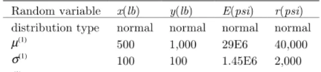
Table 1 The statistics of the random variables used in Example 1

Random variable x(lb) y(lb) E(psi) r(psi) distribution type normal normal normal normal

µ(1)

500 1,000 29E6 40,000

σ(1)

100 100 1.45E6 2,000

(1)_µ_{is the mean value and}_σ_{is the standard deviation}

x

y

b

h

(9)

4.1.1 Case 1

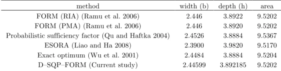
Four different RBDO algorithms were used to solve this case: the double-loop approach using SQP as the optimizer and using FORM for reliability analysis (D–SQP–FORM), the double-loop approach using SQP as the optimizer and using MCS for reliability analysis (D–SQP–MCS), the single-loop approach using SQP as the optimizer and using EPM for reliability analysis (S–SQP– EPM) and the single-loop approach using PSO as the optimizer and using EPM for reliability analysis (S–PSO–EPM). Because the current problem does not have a local optimal point and the constraint is linear, the D–SQP–FORM should deliver an accurate and identical solution given different initial points. Thus, the solution of D–SQP–FORM was used as the benchmark design. To demonstrate this idea, 9 different values of 1, 2, 3,…, 9 for each design variable were chosen, resulting in 81 initial points that were used in the D–SQP–FORM approach. These 81 optimal values, as expected, are identical, and they are 9.520246 with b= 2.44599 and h = 3.892185. These results are similar to the results from Liao and Ha (2008), Wu et al. (2001), Ramu et al. (2006) and Qu and Haftka (2004), which are shown in Table 2.

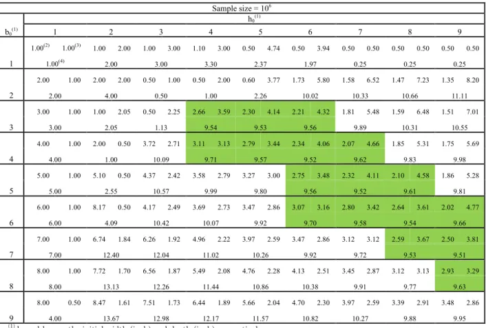
Although MCS with sufficient sample size is often considered a suitable tool for reliability analysis, it is not an easy task to completely eliminate the effect of the inherit statistic uncertain-ties of MCS on an RBDO solution (Liao and Lu 2012). To investigate this effect, D–SQP–MCS was used to solve the current RBDO problem. The same 81 initial points were used for the D– SQP–MCS approach. For each initial point, the D–SQP–MCS method was performed twice. That is, this problem was analyzed 162 times. Ideally, the goal of an optimization algorithm is to deli-ver an identical and accurate solution given different initial points. Howedeli-ver, an RBDO problem either has a local minimum or has a nonlinear constraint. In this case, it is very difficult to achieve this goal. Instead, if the difference between a solution and the "target solution" is less than 2% of the optimal solution, that solution is considered as a "reasonable solution" in current study. The "target solution" for the current problem is the solution from D–SQP–FORM in which the objective value is 9.5202. Based on this definition, Tables 3 and 4 shows that D–SQP– MCS only delivered 19 and 17 reasonable solutions (the number of green blocks), respectively. The sample size used in these analyses is 106. With this sample size, the effect of statistical uncer-tainty on an RBDO solution cannot be removed. To further investigate the influence of the sta-tistical uncertainty, other sample sizes such as 103, 104 and 105 are used for MCS. The results are displayed in Table 5. The number of reasonable solutions did not significantly increase when a greater sample size was used.

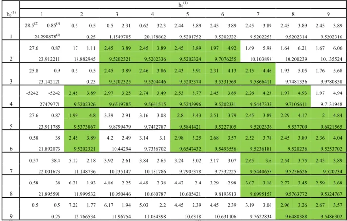
Unlike the MCS, there is no statistic uncertainty in the reliability evaluation by using EPM incorporated with GKQ. It is of interest to investigate the sensitivity of the S–SQP–EMP solu-tion with respect to the initial point. The results of S–SQP–EMP approach are displayed in Table 6. There were 36 reasonable solutions. Compared to the approach of D–SQP–MCS, the S–SQP– EMP approach is apparently less sensitive to the initial point. Thus, S–SQP–EMP is a more sta-ble RBDO approach.

(10)

coeffi-Latin American Journal of Solids and Structures 11 (2014) 826-847

cient of variation (cov) in solutions decreased from 0.038 to 0.013. In addition, the RBDO solu-tion is not significantly affected by statistic uncertainty when the sample size is greater than 103. However, greater sample size does not always produce more reasonable solutions, as shown in Table 5. Thus, the capability of delivering a reasonable solution for D–SQP–MCS depends on both the sample size and location of initial point. As results shown in Tables 5 and 7, one can conclude that the impact of initial point is significantly. No deviation among the 20 S–SQP–EMP solutions is found. Thus, it is confirmed that S–SQP–EMP is a more stable RBDO algorithm than D–SQP–MCS.

Table 2 Comparison of optimal designs among several studies (Example 1 – case 1)

method width (b) depth (h) area

FORM (RIA) (Ramu et al. 2006) 2.446 3.8922 9.5202

FORM (PMA) (Ramu et al. 2006) 2.446 3.8920 9.5202

Probabilistic sufficiency factor (Qu and Haftka 2004) 2.4526 3.8884 9.5367

ESORA (Liao and Ha 2008) 2.3900 3.9820 9.5170

Exact optimum (Wu et al. 2001) 2.4484 3.8884 9.5204

D–SQP–FORM (Current study) 2.44599 3.892185 9.5202

Table 3 Solutions from 81 different initial points using D–SQP–MCS (Example 1 – case 1, the 1st trial)

Sample size = 106

b0(1)

h0(1)

1 2 3 4 5 6 7 8 9

1

1.00(2) _1.00(3) _1.00 _2.00 _1.00 _3.00 _0.50 _3.60 _0.60 _4.84 _0.60 _3.87 _0.50 _0.50 _0.60 _0.50 _0.50 _6.89

1.00(4) _2.00 _3.00 _1.80 _2.91 _2.32 _0.25 _0.30 _3.44

2

2.00 1.00 2.00 2.00 0.50 3.17 0.50 2.00 0.50 3.00 1.75 5.69 1.68 6.01 1.48 7.20 1.39 7.88

2.00 4.00 1.58 1.00 1.50 9.98 10.11 10.64 10.96

3

3.00 1.00 1.00 0.50 0.50 0.50 2.66 3.59 2.21 4.32 2.05 4.71 1.79 5.54 1.64 6.25 1.45 7.39

3.00 0.50 0.25 9.54 9.55 9.64 9.92 10.22 10.73

4

4.00 1.00 2.00 0.50 3.66 2.74 3.11 3.12 2.74 3.49 2.56 3.72 1.84 5.36 1.80 5.49 1.64 6.22

4.00 1.00 10.05 9.71 9.56 9.52 9.85 9.90 10.20

5

5.00 1.00 3.00 0.50 4.34 2.43 3.27 3.00 2.80 3.43 2.73 3.50 2.39 3.98 2.02 4.77 1.76 5.65

5.00 1.50 10.54 9.81 9.58 9.56 9.52 9.66 9.96

6

6.00 1.00 6.21 0.50 5.00 2.21 4.51 2.37 3.46 2.87 3.15 3.09 2.83 3.39 2.28 4.19 2.16 4.44

6.00 3.10 11.05 10.67 9.92 9.73 9.59 9.53 9.57

7

7.00 1.00 7.15 1.78 5.77 2.02 5.02 2.20 4.14 2.51 3.47 2.86 2.95 3.26 3.01 3.22 2.50 3.81

7.00 12.71 11.65 11.06 10.39 9.92 9.64 9.66 9.52

8

8.00 1.00 7.58 1.72 6.55 1.87 5.74 2.03 4.03 2.56 3.71 2.72 3.48 2.85 3.12 3.12 2.85 3.37

8.00 13.02 12.25 11.63 10.31 10.09 9.93 9.71 9.60

9

8.00 0.50 8.51 1.61 7.53 1.72 6.41 1.90 5.53 2.07 4.69 2.30 4.03 2.56 3.40 2.91 2.35 4.06

4.00 13.69 12.99 12.15 11.46 10.81 10.31 9.88 9.52

(1)_b

(11)

(4)

the obtained optimal area (inch2) for the corresponding initial point

Although S–SQP–EMP is more stable than D–SQP–MCS, the stability of S–SQP–EMP still needs to be improved. As shown in Table 6, there are still 45 unreasonable solutions when using the S–SQP–EMP approach. To investigate further, three arbitrary points, (2.45, 3.90), (2.0, 3.0) and (1.0, 2.0), are selected to perform the reliability analysis using FORM, MCS and EPM. Table 8 shows that, for the point (2.45, 3.90), EPM generally delivered more promising solutions com-pared to MCS. To be specific, EPM with three moments has a better reliability evaluation than MCS with a sample size of 107. MCS with a sample size that is less than 105 is more efficient than EPM. However, their evaluations were relatively inaccurate.

In the case of point (2.0, 3.0), only the D–SQP–MCS failed to deliver a reasonable solution (Tables 3, 4 and 6). Table 9 displays the failure probability and the gradient with respect to the horizontal force (x) for the approaches of FORM, MCS and EPM. For the failure probability, all three approaches were very close. Because a gradient-based optimizer (SQP) is used at this stage, it is worth examining the gradients of the three approaches at this point. The MCS gradient was apparently different than the gradients of the other two approaches. Thus, for this particular point, the inaccurate gradient information calculated by MCS may result in an unreasonable solu-tion for the D–SQP–MCS approach.

Table 4 Solutions from 81 different initial points using D–SQP–MCS (Example 1 – case 1, the 2nd trial)

Sample size = 106

b0(1)

h0(1)

1 2 3 4 5 6 7 8 9

1

1.00(2) 1.00(3) 1.00 2.00 1.00 3.00 1.10 3.00 0.50 4.74 0.50 3.94 0.50 0.50 0.50 0.50 0.50 0.50

1.00(4) 2.00 3.00 3.30 2.37 1.97 0.25 0.25 0.25

2

2.00 1.00 2.00 2.00 0.50 1.00 0.50 2.00 0.60 3.77 1.73 5.80 1.58 6.52 1.47 7.23 1.35 8.20

2.00 4.00 0.50 1.00 2.26 10.02 10.33 10.66 11.11

3

3.00 1.00 1.00 2.05 0.50 2.25 2.66 3.59 2.30 4.14 2.21 4.32 1.81 5.48 1.59 6.48 1.51 7.01

3.00 2.05 1.13 9.54 9.53 9.56 9.89 10.31 10.55

4

4.00 1.00 2.00 0.50 3.72 2.71 3.11 3.13 2.79 3.44 2.34 4.06 2.07 4.66 1.85 5.31 1.75 5.69

4.00 1.00 10.09 9.71 9.57 9.52 9.62 9.83 9.98

5

5.00 1.00 5.10 0.50 4.37 2.42 3.58 2.79 3.27 3.00 2.75 3.48 2.32 4.11 2.10 4.58 1.86 5.28

5.00 2.55 10.57 9.99 9.80 9.56 9.52 9.61 9.81

6

6.00 1.00 8.17 0.50 4.17 2.49 3.69 2.73 3.47 2.86 3.07 3.16 2.80 3.42 2.64 3.61 2.02 4.77

6.00 4.09 10.42 10.07 9.92 9.70 9.58 9.54 9.66

7

7.00 1.00 6.74 1.84 6.26 1.92 4.96 2.22 3.97 2.59 3.47 2.86 3.12 3.12 2.59 3.67 2.50 3.81

7.00 12.40 12.04 11.02 10.26 9.92 9.72 9.53 9.51

8

8.00 1.00 7.72 1.70 6.56 1.87 5.49 2.08 4.76 2.28 4.13 2.51 3.45 2.87 3.12 3.13 2.93 3.29

8.00 13.13 12.26 11.44 10.86 10.38 9.91 9.77 9.63

9

8.00 0.50 8.47 1.61 7.51 1.73 6.44 1.89 5.66 2.04 4.70 2.30 3.97 2.59 3.39 2.91 3.48 2.86

4.00 13.67 12.98 12.17 11.57 10.82 10.27 9.88 9.95

(1) _b

(12)

(4) _{the obtained optimal area (inch}2_{) for the corresponding initial point}

Table 5 Number of reasonable solutions for D–SQP–MCS and S–SQP–EMP (Example 1 – case 1)

RBDO approach No. of reasonable solution 1st trial 2nd trial

S–SQP–EMP 36 -

D–SQP–MCS (sample size = 106) 19 17

D–SQP–MCS (sample size = 105₎ ₁₉ ₁₉

D–SQP–MCS (sample size = 104₎ ₁₇ ₁₇

Table 6 Solutions from 81 different initial points using S–SQP–EMP (Example 1 – case 1)

b0(1)

h0(1)

1 2 3 4 5 6 7 8 9

1

28.5(2) 0.85(3) 0.5 0.5 0.5 2.31 0.62 32.3 2.44 3.89 2.45 3.89 2.45 3.89 2.45 3.89 2.45 3.89

24.290878(4) 0.25 1.1549705 20.178862 9.5201752 9.5202322 9.5202255 9.5202314 9.5202316

2

27.6 0.87 17 1.11 2.45 3.89 2.45 3.89 2.45 3.89 1.97 4.92 1.69 5.98 1.64 6.21 1.67 6.06

23.912211 18.882945 9.5202321 9.5202336 9.5202324 9.7076255 10.103898 10.200239 10.135524

3

25.8 0.9 0.5 0.5 2.45 3.89 2.46 3.86 2.43 3.91 2.31 4.13 2.15 4.46 1.93 5.05 1.76 5.68

23.142121 0.25 9.5202325 9.5204446 9.5203374 9.5331569 9.5866411 9.7481336 9.9780858

4

-5242 -5242 2.45 3.89 2.97 3.25 2.74 3.49 2.53 3.77 2.45 3.89 2.26 4.23 1.97 4.93 1.97 4.94

27479771 9.5202326 9.6519785 9.5661515 9.5243996 9.5202331 9.5447335 9.7105611 9.7131948

5

27.6 0.87 1.99 4.8 3.39 2.91 3.16 3.08 2.8 3.43 2.51 3.79 2.45 3.89 2.29 4.17 2 4.84

23.911785 9.5373867 9.8799479 9.7472787 9.5841421 9.5227105 9.5202336 9.537709 9.6821565

6

0.58 38 2.45 3.89 4.2 2.49 3.14 3.1 2.98 3.25 2.68 3.57 2.52 3.78 2.45 3.89 2.36 4.04

21.892073 9.5202321 10.44294 9.7336702 9.6547432 9.5493556 9.5236181 9.520236 9.5253702

7

0.57 38.4 5.12 2.18 3.92 2.61 3.84 2.65 3.24 3.02 3.17 3.07 2.65 3.6 2.54 3.75 2.45 3.89

22.001673 11.148736 10.235147 10.181786 9.7905378 9.7532225 9.5440655 9.5256626 9.520234

8

0.58 38 6.21 1.93 4.86 2.25 4.49 2.38 4.42 2.4 3.29 2.98 3.07 3.16 2.77 3.45 2.59 3.68

21.895591 11.999532 10.950446 10.660787 10.605421 9.8193913 9.6995157 9.5763772 9.5324767

9

0.5 0.5 7.22 1.77 6.17 1.94 5.03 2.2 4.45 2.39 4.45 2.39 3.19 3.06 2.96 3.26 2.67 3.57

0.25 12.766534 11.96754 11.084398 10.6318 10.631106 9.7622834 9.6480388 9.5486302 (1) _b

0and h0 are the initial width (inch) and depth (inch), respectively, (2) the obtained optimal width (inch) for the correspon-ding initial point, (3) the obtained optimal depth (inch) for the corresponding initial point, (4)the obtained optimal area (inch2) for the corresponding initial point

(13)

provided an approximated reliability but incorrect gradient information. Thus, both D–SQP– MCS and S–SQP–EPM failed to deliver an accurate RBDO solution.

Based on results found in Tables 8, 9 and 10, if the point is located near the "target solution" or in the feasible domain, the chance to deliver a reasonable solution is higher for the D–SQP– MCS and S–SQP–EPM approaches. However, if the point is located in the infeasible domain, the above two approaches often fail to deliver a reasonable solution due to an inaccurate evaluation of the reliability and the gradient. In addition, the statistic uncertainty has a significant impact on the stability of an RBDO solution, and thus D–SQP–MCS delivers a less reasonable solution than S–SQP–EPM.

EPM is generally a more efficient method for reliability evaluation compared to MCS. However, if the design point is located in the infeasible region, EPM combined with SQP often fails to find a good RBDO solution. In this case, this study suggests the use of another optimizer (PSO) to conduct the optimization to consistently deliver an optimal solution.

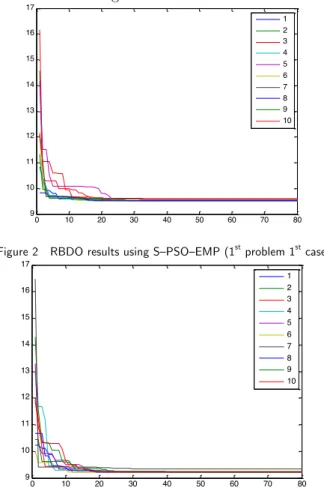
To prevent the particle from being trapped in a local minimum, a space-filling experiment de-sign (i.e., the Latin hypercube) is used to generate the first generation of the particles in PSO. Because PSO is a population-based algorithm, S–PSO–EPM was performed 10 times to display the variation among solutions. Thirty particles and 80 iterations were used in PSO for the current study. The statistics of the S–PSO–EPM solutions are displayed in Table 11. The history of the objective value for 10 runs is shown in Figure 2. As shown in Figure 2, for most analysis repeti-tions, the alteration of the global best after the 40th iteration is very small. Compared with the "target solution" (9.520246), all of the results of the S–PSO–EPM analysis were within a range of less than 1% deviation. That is, all solutions can be considered as a reasonable solution, indica-ting that the PSO algorithm is perfectly integrated with the EPM. S–PSO–EPM was thus shown to be able to consistently deliver an optimal solution and thus is a stable RBDO algorithm.

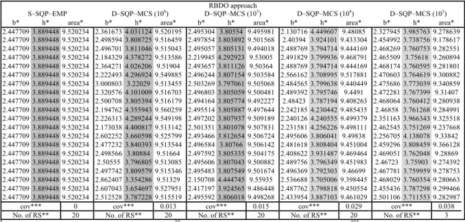
Table 7 20 solutions using identical initial point (7, 9) from D–SQP–MCS & S–SQP–EMP (Example 1 – case 1)

RBDO approach

S–SQP–EMP D–SQP–MCS (106₎ _{D–SQP–MCS (10}5₎ _{D–SQP–MCS (10}4₎ _{D–SQP–MCS (10}3₎

b* h* area* b* h* area* b* h* area* b* h* area* b* h* area*

2.447709 3.889448 9.520234 2.361673 4.031124 9.520195 2.495304 3.80554 9.495981 2.130716 4.449607 9.48085 2.327945 3.985763 9.278639 2.447709 3.889448 9.520234 2.498594 3.808725 9.516459 2.497854 3.803892 9.501568 2.40394 3.924101 9.433304 2.454992 3.738756 9.178617 2.447709 3.889448 9.520234 2.496701 3.811046 9.515043 2.495057 3.805131 9.494018 2.488769 3.794714 9.444169 2.468269 3.760753 9.282551 2.447709 3.889448 9.520234 2.184329 4.378272 9.513586 2.219945 4.292923 9.53005 2.491829 3.799936 9.468791 2.465509 3.75618 9.260894 2.447709 3.889448 9.520234 2.364271 4.026206 9.51904 2.493657 3.811126 9.50364 2.488769 3.794714 9.444169 2.468174 3.760595 9.281801 2.447709 3.889448 9.520234 2.222493 4.296924 9.549885 2.496244 3.807154 9.503584 2.566162 3.708995 9.517881 2.470603 3.764619 9.300882 2.447709 3.889448 9.520234 3.000803 3.22029 9.513455 2.503269 3.797061 9.505068 2.484565 3.799638 9.440449 2.475686 3.773039 9.340859 2.447709 3.889448 9.520234 2.320576 4.101009 9.516703 2.496803 3.805059 9.500481 2.489392 3.795746 9.4491 2.472281 3.767399 9.31407 2.447709 3.889448 9.520234 2.500708 3.805394 9.516179 2.494164 3.805774 9.492227 2.48423 3.787194 9.408263 2.468064 3.760412 9.280938 2.447709 3.889448 9.520234 2.194762 4.355943 9.560259 2.495514 3.805887 9.497644 2.242185 4.230442 9.485435 2.46858 3.761268 9.284991 2.447709 3.889448 9.520234 2.226313 4.289244 9.549198 2.497202 3.807937 9.509189 2.240126 4.240555 9.499379 2.351163 3.966343 9.325518 2.447709 3.889448 9.520234 2.173038 4.400817 9.513142 2.501351 3.801078 9.507831 2.231581 4.256226 9.498111 2.462545 3.751269 9.237668 2.447709 3.889448 9.520234 2.602252 3.660598 9.525799 2.493466 3.812654 9.506724 2.495606 3.806041 9.49838 2.256705 4.138078 9.33842 2.447709 3.889448 9.520234 2.477232 3.840393 9.513544 2.496584 3.80766 9.506142 2.481618 3.808404 9.451004 2.459296 3.808459 9.366128 2.447709 3.889448 9.520234 2.498566 3.80884 9.51664 2.497592 3.805335 9.504175 2.408622 3.931487 9.469464 2.469051 3.762048 9.28869 2.447709 3.889448 9.520234 2.50555 3.796805 9.513085 2.495606 3.807043 9.500882 2.489756 3.796349 9.451983 2.46723 3.75903 9.274392 2.447709 3.889448 9.520234 2.497742 3.809579 9.515346 2.495483 3.807549 9.501674 2.496369 3.792303 9.46699 2.467781 3.759959 9.278753 2.447709 3.889448 9.520234 2.862407 3.354286 9.51329 2.150708 4.444745 9.55935 2.536688 3.705006 9.398445 2.468029 3.760354 9.280663 2.447709 3.889448 9.520234 2.607043 3.654697 9.527951 2.417197 3.924565 9.486448 2.487762 3.798818 9.450554 2.455436 3.787298 9.299466 2.447709 3.889448 9.520234 2.512528 3.787228 9.515519 2.495592 3.806018 9.498268 2.433954 3.887103 9.461029 2.501106 3.711553 9.282987

cov*** 0 cov*** 0.013 cov*** 0.015 cov*** 0.029 cov*** 0.038

(14)

Latin American Journal of Solids and Structures 11 (2014) 826-847 Table 8 15 reliability evaluations using FORM, MCS & EMP for the point of (2.45, 3.90)

Table 9 Ten reliability and gradient evaluations using FORM, MCS & EMP for the point of (2.0, 3.0)

Table 10 Reliability and gradient evaluations using FORM, MCS & EMP for the point of (1.0, 2.0)

*mean value of 10 runs

Table 11 Statistics of using S–PSO–EMP to solve Example 1 – case 1 problem

No. FORM

MCS EPM

103 104 105 106 107 Moment

= 3

Moment = 4

Moment = 5

Moment = 6 1

0.9988752

0.999 0.99920 0.99905 0.998908 0.9988688

0.9988752 0.9988752 0.9988752 0.9988752

2 1.000 0.99860 0.99904 0.998866 0.998876

3 0.999 0.99960 0.99902 0.998881 0.9988893

4 1.000 0.99910 0.99894 0.998823 0.998891

5 0.999 0.99900 0.99884 0.998889 0.9988696

6 0.997 0.99860 0.99881 0.998858 0.9988962

7 0.999 0.99920 0.99868 0.998865 0.9988952

8 1.000 0.99900 0.99892 0.998877 0.998869

9 1.000 0.99950 0.99894 0.998874 0.9988811

10 0.998 0.99890 0.99879 0.998855 0.9988817

11 1.000 0.99840 0.99903 0.998875 0.9988708

12 1.000 0.99880 0.99899 0.998885 0.9988783

13 1.000 0.99880 0.99884 0.998846 0.9988565

14 0.999 0.99830 0.99905 0.99888 0.9988658

15 0.998 0.99880 0.99893 0.998864 0.9988733

mean 0.9992 0.99892 0.99892 0.998870 0.9988775

standard

deviation – 0.000941 0.0003687 0.0001118

1.994E-05

1.155E-05 – – – –

Time

(seconds) – 0.000480 0.001553 0.013889 0.077984 0.741181 0.036613 0.041205 0.060109 0.065282

No. FORM MCS (107) EPM abs(FORM -

MCS)/FORM

abs(FORM - EPM)/FORM

gradient 1

0.038358663537357

0.038292000000000

0.038358663612451

0.001738

1.95768E-09

2 0.037997000000000 0.009428

3 0.038125999999999 0.006065

4 0.038047999999999 0.008099

5 0.038210000000001 0.003876

6 0.038665999999999 0.008012

7 0.038138000000000 0.005753

8 0.038062000000000 0.007734

9 0.038546000000000 0.004884

10 0.038345000000000 0.000356

failure probability 0.998102617416204 0.998114000000000 0.998102618399013 – –

No. FORM MCS (107₎ _EPM

(15)

Mean Standard Dev. Min. Value Max. Value

9.55249 0.035535 9.5203 9.6067

4.1.2 Case 2

In contrast to the stress limit state problem considered in the first case, the second case is a non-linear problem. In this situation, no analytical reliability analysis is available. To examine the stability of an RBDO algorithm, the optimal point (2.721, 3.392) from Liao and Ha (2008) is used as the target solution instead of using the D–SQP–FORM solution. Both S–SQP–EPM and D– SQP–MCS (with sample sizes of 103, 104, 105 and 106) were used to solve the current RBDO task using 81 identical initial points, as explained in the previous section. Similarly, D–SQP–MCS was conducted twice for each initial point. The summary of the number of reasonable solutions is dis-played in Table 12. When the limit state function is nonlinear, S–SQP–EPM still delivers more reasonable solutions than D–SQP–MCS. The number of reasonable solutions is moderately affec-ted by the sample size. The results of using S–PSO–EPM are provided in Table 13 and Figure 3. The solutions converged at approximately 30 iterations. In addition, all optimal points were a reasonable solution. For the case of the nonlinear limit state function, S–PSO–EPM was able to deliver a consistent RBDO solution among the different trials.

Figure 2 RBDO results using S–PSO–EMP (1st problem 1st case)

Figure 3 RBDO results using S–PSO–EMP (1st problem 2nd case)

0 10 20 30 40 50 60 70 80

9 10 11 12 13 14 15 16 17

1 2 3 4 5 6 7 8 9 10

0 10 20 30 40 50 60 70 80

9 10 11 12 13 14 15 16 17

1

2

3 4

5

6

7

8 9

(16)

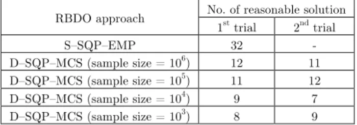
Latin American Journal of Solids and Structures 11 (2014) 826-847 Table 12 Number of reasonable solutions for D–SQP–MCS and S–SQP–EMP (Example 1 – case 2)

S–SQP–EMP 32 -

Table 13 Statistics of using S–PSO–EMP to solve Example 1 – case 2 problem

Mean Standard Dev. Min. Value Max. Value

9.23735 0.0356 9.2216 9.3376

4.2 A three bar truss problem

The second example is a three bar truss problem, that is adopted from Thanedar and Kodiyalam (1992), displayed in Figure 4. The statistics of the random parameters are displayed in Table 14. The optimization formulation is shown below.

minimize W=(2 2A₁+A₂)

s.t. G₁: Prob.( 2Pxl A₁E

−δ

a≤0)≥0.9772

G₂: Prob.( 2Pyl (A₁+ 2A₂)E

−δ

a≤0)≥0.9772

G₃: | 1 2[

P_x A₁+

P_y

(A₁+ 2A₂)]| ≤₅₀₀₀

G₄: | 2Py (A₁+ 2A₂)|

≤₂₀₀₀₀

G₅: | 1 2[

P_y

(A₁+ 2A₂) − Px

A₁]| ≤₅₀₀₀

0.1≤_A

i, i=1, 2, 3

(16)

where W is the total weight of the structure, A1 is the cross-sectional area for members 1 and 3 (inch2), A2 is the cross-sectional area for member 2 (inch2), Px ( 10000 2lbs) and Py ( 20000 2lbs)

(17)

ensure that the resulting compressive/tensile stresses for members 1, 2 and 3 are less than 5000 psi, 20,000 psi and 5000 psi, respectively.

Figure 4 A three bar truss used in the second example

Similar to the first example, this example was analyzed 81 times using different initial points for both the D–SQP–MCS and S–SQP–EPM approaches. The initial point is a pair (Ai, Aj), whe-re Ai and Aj are values of 1, 2, 3,…, 9, resulting in 81 different points. Because the probability density function (PDF) is not provided in the literature study of Thanedar and Kodiyalam (1992), this study assumes that all random parameters follow a normal distribution, as shown in Table 14. The "target solution" is defined as the "best solution" among the 81 S–SQP–EPM solutions, and it is 21.112 with a design point of 6.31 and 3.265, as indicated in Table 15. The reliability analysis at the "target solution" was conducted, and the result is displayed in Table 15. It is clear that the "target solution" satisfied the reliability requirement. The number of reasonable solutions for D–SQP–MCS and S–SQP–EPM are provided in Table 16. The statistical uncertainty produced by the MCS results in a very unstable solution for the D–SQP–MCS approach. Although increa-sing the sample size can effectively reduce the variation in the number of reasonable solutions, it does not promise to have a greater number of reasonable solutions. S–SQP–EPM certainly domi-nated over D–SQP–MCS in terms of solution stability for any sample size.

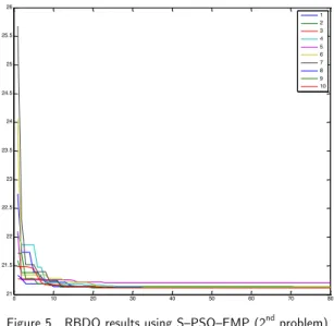
The results of using S–PSO–EPM for the second problem are provided in Table 17 and Figure 5. The range for the 10 solutions was from 21.112 to 21.201. None of these solutions has a devia-tion that is larger than 2% from the "target soludevia-tion" (21.112), indicating that S–PSO–EPM is a suitable and stable optimization algorithm.

10” 10”

10”

1 2 3

Px

(18)

Figure 5 RBDO results using S–PSO–EMP (2nd problem)

Table 14 The statistics of the random variables used in Example 2

Random variable E(psi) δα

(2)₍ inch) distribution type normal normal

µ(1)

1.0E7 0.005

cov 0.1 0.1

(1)_{is the mean value}

(2)_{is the allowable displacement in both}

x and y direction

Table 15 Optimal point and its reliability analysis for the 2nd problem

Optimal design (6.31,

3.265) Reliability value for the x direction 0.9977 Reliability value for the y direction 0.9772

Table 16 Number of reasonable solutions for D–SQP–MCS and S–SQP–EMP (Example 2)

S–SQP–EMP 74 -

D–SQP–MCS (sample size = 104₎ ₄₉ ₃₈

Table 17 Statistics of using S–PSO–EMP to solve Example 2

Mean Standard Dev. Min. Value Max. Value 21.128 0.027 21.112 21.201

0 10 20 30 40 50 60 70 80

21 21.5 22 22.5 23 23.5 24 24.5 25 25.5 26

(19)

4.3 A mathematical problem with multiple limit states

The mathematical formulation of this problem, adopted from Youn and Choi (2004), is provided in Equation (17).

Min. f(D)=(D₁+D₂)

s.t. prob(G_j(P)≥0)≥97.72%, j=1 ~ 3

-10≤D_i≤10, i=1 ~ 2

where G₁(P)=1-P₁2 P₂/ 20

G₂(P)=1−(P₁+P₂−5)2/ 30

−(P₁-P₂−12)2

/ 120

G₃(P)=1−80 / (P₁2

+8P₂+5)

(17)

where D _{are the design variables, which}_{are the mean values of the random design variables (}P₎_, in which P_{~ N (}D_{, 0.6}2_)._G_{i is the}_ith_{constraint. The target reliability is 97.72% (}_β_{= 2)} _{for all} three constraints. In contrast to the first two problems, a system reliability problem is involved in this RBDO task. Similar to the second example, the "target solution" is defined as the "best solu-tion" among the 81 S–SQP–EPM solutions, and it is 7.265 with 3.653 and 3.612 for D1 and D2, respectively. A comparison between the target solution and the solutions from Youn and Choi (2004) is provided in Table 18. The suitability of the target solution used here is thus confirmed.

Similar to the first two examples, both S–SQP–MCS and S–SQP–EPM were performed 81 ti-mes. The number of reasonable solutions for each approach is displayed in Table 19. With respect to the stability, S–SQP–EPM is a better RBDO approach, which is confirmed in this example. S– PSO–EPM was conducted to further improve the stability of the calculated solutions. The results of S–PSO–EPM are provided in Table 20 and Figure 6. The 10 solutions from S–PSO–EPM were all 7.2652. This solution only deviated 0.000275% from the target solution, indicating that S– PSO–EPM is able to consistently provide an accurate RBDO solution.

Figure 6 RBDO results using S–PSO–EMP (3rd problem)

0 10 20 30 40 50 60 70 80

7 7.5 8 8.5 9 9.5 10 10.5 11 11.5

(20)

Latin American Journal of Solids and Structures 11 (2014) 826-847 Table 18 Comparison of optimal design between current study and literature study

Method d1 d2 objective

RIA (Youn and Choi 2004) 3.609 3.661 7.27 PMA (Youn and Choi 2004) 3.609 3.660 7.269

S–SQP–EMP 3.653 3.612 7.265

Table 19 Number of reasonable solutions for D–SQP–MCS and S–SQP–EMP (Example 3)

S–SQP–EMP 47 -

D–SQP–MCS (sample size = 103₎ ₅ ₅

Table 20 Statistics of using S–PSO–EMP to solve Example 3

Mean Standard Dev. Min. Value Max. Value 7.2652 0.00 7.2652 7.2652

5 CONCLUSIONS

This study integrates EPM with SQP or PSO to formulate an RBDO algorithm and emphasizes its ability of solving a nonlinear RBDO problem accurately and consistently. MCS with a suffi-cient sample size is often used for reliability evaluation in nonlinear cases. This study shows that EPM is a better approach than MCS in terms of accuracy and efficiency. Integrating MCS with SQP often fails to deliver a consistent RBDO solution due to the inherit statistical uncertainty in MCS. Both of the proposed approaches, S–SQP–EPM and S–PSO–EPM, possess a better stabili-ty performance than D–SQP–MCS. By performing an RBDO using the proposed method, the reliability analysis at each design point was evaluated through EPM, where only a single iteration is needed and therefore the proposed algorithm can be considered as a single loop RBDO ap-proach.

(21)

do-Latin American Journal of Solids and Structures 11 (2014) 826-847

main, LHS was implemented in PSO. Some conclusions are drawn below according to the results obtained.

1. Compared to MCS with a sample size of 107, EPM is able to compute the reliability more effi-ciently with the same accuracy.

2. The effect of the statistical uncertainty on an RBDO solution is significantly, which was de-monstrated by the stability performance of D–SQP–MCS.

3. S–PSO–EPM is able to consistently deliver a promising result in which the deviation from the target solution is often less than 2%. Thus, S–PSO–EPM is the most stable RBDO algorithm among all of the approaches examined in this study.

In this study, the stability, accuracy and efficiency of S–PSO–EPM are examined by three RBDO problem that only have two design variables. Because S–PSO–EPM is a population-based algorithm, its efficiency decreases as the problem size increases. For example, a larger problem usually requires a larger population size so as to delay the solution convergence. On the other hand, similar to the standard PSO, the stability and accuracy of S–PSO–EPM is not largely af-fected by the problem size. Since this study focuses more on locating the global optimum consis-tently than obtaining a fast solution, certain compensation in efficiency is needed. However, if the efficiency is a major concern, the proposed S–PSO–EPM is suitable for parallel computing and thus, the computational cost can be alleviated.

Acknowledgements This study was supported by National Science Council of Taiwan under grant number 100WFA2500489. The support is gratefully acknowledged.

References

Aoues, Y., Chateauneuf, A., (2010). Benchmark study of numerical methods for reliability-based design opti-mization. Structural and Multidisciplinary Optimization 41(2): 277–294.

Beck, A.T., Verzenhassi, C.C., (2008). Risk optimization of a steel frame communications tower subject to tornado winds. Latin American Journal of Solids and Structures 5(3): 187–203.

Chen, X., Hasselman, T.K., Neill, D.J., (1997). Reliability based structural design optimization for practical applications. Proceedings of the 38th AIAA/ASME/ASCE/AHS/ASC Structures, Structural Dynamics, and Materials Conference, Kissimmee, FL, Paper No. AIAA-97-1403.

Du, X., Chen, W., (2003). Sequential optimization and reliability assessment method for efficient probabilistic design. J. of Mechanical Design 126(2): 225–233.

Er, G.K. (1998). A method for multi-parameter PDF estimation of random variables. Structural Safety 20: 25– 36.

Kaymaz, I., Marti, K., (2007). Reliability-based design optimization for elastoplastic mechanical structures. Computers & Structures 85(10): 615–625.

Li, F., Wu, T., Hu, M., Dong, J., (2010). An accurate penalty-based approach for reliability-based design op-timization. Research in Engineering Design 21(2 ): 87–98.

Liang, J.h., Mourelatos, Z.P., Nikolaidis, E., (2007). A single-loop approach for system reliability-based design optimization. J. of Mechanical Design 129: 1215–91224.

(22)

Liao, K.W., Lu, H., (2012). An iterative topology optimization algorithm that considers randomness in design parameters. J. of Advanced Mechanical Design, Systems, and Manufacturing 6(7): 1319–1336.

Liao, K.W., Lu, H., (2012). A stability investigation of a simulation- and reliability-based optimization. Struc-tural and Multidisciplinary Optimization 46(5): 761–781.

Parsopoulos, K.E., Vrahatis, M.N., (2002). Particle swarm optimization method for constrained optimization problems. Intelligent Technologies–Theory and Application: New Trends in Intelligent Technologies 76: 214– 220.

Qu, X., Haftka, R.T., (2004). Reliability-based design optimization using probabilistic sufficiency factor. Structural and Multidisciplinary Optimization 27(5): 314–325.

Ramu, P., Qu, X., Youn, B.D., Haftka, R.T., (2006). Inverse reliability measures and reliability-based design optimisation. International Journal of Reliability and Safety 1: 187–205.

Ramu, P., Qu, X., Youn, B.D., Haftka, R.T., Choi, K.K., (2004). Safety factor and inverse reliability measures. Proceeding of 45th AIAA/ASME/ASCE/AHS/ASC Structures, Structural Dynamics and Materials Conference, Palm Springs, California, Paper No. AIAA-2004-1670.

Shan, S., Wang, G.G., (2008). Reliable design space and complete single-loop reliability-based design optimiza-tion. Reliability Engineering & System Safety 93(8): 1218–1230.

Thanedar, P.B., Kodiyalam, S., (1992). Structural optimization using probabilistic constraints. Structural and Multidisciplinary Optimization 4: 236–240.

Tu, J., Choi, K.K., Park, Y.H., (2001). Design potential method for robust system parameter design. AIAA Journal 39(4): 667–677.

Wu, Y.T., Shin, Y., Sues, R., Cesare, M., (2001). Safety-factor based approach for probability-based design optimization. Proceedings of the 42rd AIAA/ASME/ASCE/AHS/ASC Structures, Structural Dynamics, and Materials Conference, Paper No. AIAA-2001-1522.

Youn, B.D., Choi, K.K., (2004). An investigation of nonlinearity of reliability based design optimization ap-proaches. J. of Mechancial Design 26(3):403–411.