Aerosol-climate interactions in the Norwegian Earth System Model – NorESM

(1)

GMDD

5, 2599–2685, 2012

Aerosol-climate interactions in the

Norwegian Earth System Model

A. Kirkev ˚ag et al.

Title Page

Abstract Introduction

Conclusions References

Tables Figures

◭ ◮

Back Close

Full Screen / Esc

Printer-friendly Version Interactive Discussion

Discussion

P

a

per

|

Dis

cussion

P

a

per

|

Discussion

P

a

per

|

Discussio

n

P

a

per

Geosci. Model Dev. Discuss., 5, 2599–2685, 2012 www.geosci-model-dev-discuss.net/5/2599/2012/ doi:10.5194/gmdd-5-2599-2012

Geoscientific Model Development Discussions

This discussion paper is/has been under review for the journal Geoscientific Model Development (GMD). Please refer to the corresponding final paper in GMD if available.

Aerosol-climate interactions in the

Norwegian Earth System Model – NorESM

A. Kirkev ˚ag1, T. Iversen1,2, Ø. Seland1, C. Hoose2,3, J. E. Kristj ´ansson2,

H. Struthers4,5, A. M. L. Ekman5, S. Ghan6, J. Griesfeller1, E. D. Nilsson4, and

M. Schulz1

1

Norwegian Meteorological Institute, Oslo, Norway 2

Department of Geosciences, University of Oslo, Oslo, Norway 3

Karlsruhe Institute of Technology, Institute for Meteorology and Climate Research, Karlsruhe, Germany

4

Department of Applied Environmental Science, Stockholm University, Stockholm, Sweden 5

Department of Meteorology, Stockholm University, Stockholm, Sweden 6

Pacific Northwest National Laboratory, Richland, USA

Received: 10 July 2012 – Accepted: 26 July 2012 – Published: 3 September 2012

Correspondence to: A. Kirkev ˚ag (alf.kirkevag@met.no)

(2)

GMDD

5, 2599–2685, 2012

Title Page

Tables Figures

◭ ◮

Back Close

Full Screen / Esc

Discussion

P

a

per

|

Dis

cussion

P

a

per

|

Discussion

P

a

per

|

Discussio

n

P

a

per

|

Abstract

The objective of this study is to document and evaluate recent changes and updates to the module for aerosols and aerosol-cloud-radiation interactions in the atmospheric module CAM4-Oslo of the Norwegian Earth System Model (NorESM). Particular atten-tion is paid to the role of natural organics, sea salt, and mineral dust in determining the

5

gross aerosol properties as well as the anthropogenic contribution to these properties and the associated direct and indirect radiative forcing.

The aerosol module is extended from earlier versions that have been published, and includes life-cycling of sea-salt, mineral dust, particulate sulphate, black carbon, and primary and secondary organics. The impacts of most of the numerous changes since

10

previous versions are thoroughly explored by sensitivity experiments. The most impor-tant changes are: modified prognostic sea salt emissions; updated treatment of precip-itation scavenging and gravprecip-itational settling; inclusion of biogenic primary organics and methane sulphonic acid (MSA) from oceans; almost doubled production of land-based biogenic secondary organic aerosols (SOA); and increased ratio of organic matter to

15

organic carbon (OM / OC) for biomass burning aerosols from 1.4 to 2.6.

Compared with in-situ measurements and remotely sensed data, the new treatments of sea salt and dust aerosols give smaller biases in near surface mass concentrations and aerosol optical depth than in the earlier model version. The model biases for mass concentrations are approximately unchanged for sulphate and BC. The enhanced

lev-20

els of modeled OM yield improved overall statistics, even though OM is still underesti-mated in Europe and over-estiunderesti-mated in North America.

The global direct radiative forcing (DRF) at the top of the atmosphere has changed

from a small positive value to−0.08 W m−2 in CAM4-Oslo. The sensitivity tests

sug-gest that this change can be attributed to the new treatment of biomass burning

25

(3)

GMDD

5, 2599–2685, 2012

Title Page

Tables Figures

◭ ◮

Back Close

Full Screen / Esc

Discussion

P

a

per

|

Dis

cussion

P

a

per

|

Discussion

P

a

per

|

Discussio

n

P

a

per

surface has increased by ca. 60 %, to −1.89 W m−2. We show that this can be

ex-plained by new emission data and omitted mixing of constituents between updrafts and downdrafts in convective clouds.

The increased abundance of natural OM and the introduction of a cloud droplet spec-tral dispersion formulation are the most important contributions to a considerably

de-5

creased estimate of the indirect radiative forcing (IndRF). The IndRF is also found to be sensitive to assumptions about the coating of insoluble aerosols by sulphate and

OM. The IndRF of−1.2 W m−2, which is closer to the IPCC AR4 estimates than the

previous estimate of−1.9 W m−2, has thus been obtained without imposing unrealistic

artificial lower bounds on cloud droplet number concentrations.

10

1 Introduction

Aerosol particles scatter and absorb solar radiation and provide nuclei for condensa-tion of water and formacondensa-tion of ice in air. Thus they potentially influence the natural climate as well as climate change through human activity. The efficiency of this influ-ence depends on aerosol production, transport, and removal, and on microphysical

15

processes such as nucleation, condensation, and coagulation that determine the com-position, size, and shape of the particles. Since most of these processes are either approximately represented in global climate models or are not well known in the first place, aerosols constitute an important source of uncertainty in climate simulations and future projections. A recent overview of key challenges in understanding and modeling

20

aerosols and their e_ffects on climate and environment is given by Kulmala et al. (2011). Inter-model di_fferences, and thus climate projection uncertainty, can to a large extent be attributed to aerosol-cloud interactions and cloud feedbacks (Penner et al., 2006; Forster et al., 2007; Randall et al., 2007; Hegerl et al., 2007).

This paper describes and discusses the representation of aerosols and the

pro-25

(4)

GMDD

5, 2599–2685, 2012

Title Page

Tables Figures

◭ ◮

Back Close

Full Screen / Esc

Discussion

P

a

per

|

Dis

cussion

P

a

per

|

Discussion

P

a

per

|

Discussio

n

P

a

per

|

the CMIP5 protocol for the upcoming fifth assessment report from IPCC (Bentsen et al., 2012; Iversen et al., 2012). Model-representation of processes leading to an-thropogenic aerosol radiative forcing is described here, whilst estimates of climate response to aerosol forcing are discussed by Bentsen et al. (2012) and Iversen et al. (2012). Sand et al. (2012) present a model study on Arctic climate response to

5

remote and local forcing of black carbon, also using NorESM.

The scheme for calculating the life-cycle of aerosol particles along with their optical and physical properties is developed from the version thoroughly described by Seland et al. (2008) and Kirkev ˚ag et al. (2008). NorESM further incorporates extensions for cloud microphysics with prognostic cloud droplet number concentration (Storelvmo et

10

al., 2006; Hoose et al., 2009) and for wind-driven sea-salt emissions (Struthers et al., 2011). Changes in the NorESM aerosol module are discussed relative to these papers, in particular Seland et al. (2008). The role of natural aerosols in the earth system in general, and for modulating climate impacts of anthropogenic aerosols in particular, is emphasized.

15

NorESM is based on version 4 of the Community Climate System Model (CCSM4) developed at the US National Center for Atmospheric Research (NCAR) (Gent et al., 2011). This system’s atmospheric component, the Community Atmosphere Model ver-sion 4 (CAM4: Neale et al., 2010) is changed to include the aerosol module developed for NorESM and is referred to as CAM4-Oslo.

20

Potential climate impacts of aerosols are partly direct e_ffects linked to increased

scattering and absorption of solar radiation (e.g. Charlson et al., 1992), and partly

indirect e_ffects via induced changes in cloud microphysics. The radiative forcing of

the direct e_ffects at the top of the atmosphere can be negative or positive depending

on the relative importance of the changes in absorption and scattering. This relative

25

importance depends on the anthropogenic aerosols but also on the natural aerosols

and the albedo of the underlying surface. The indirect e_ffect of pure water clouds,

however, exerts a negative radiative forcing through increased cloud droplet number

(5)

GMDD

5, 2599–2685, 2012

Title Page

Tables Figures

◭ ◮

Back Close

Full Screen / Esc

Discussion

P

a

per

|

Dis

cussion

P

a

per

|

Discussion

P

a

per

|

Discussio

n

P

a

per

uncertainty is associated with the second indirect effect (Albrecht, 1989), associated with changes in cloud water content and cloudiness (Stevens and Feingold, 2009).

The semi-direct e_ffect is potentially positive due to decreased low level cloudiness when increased aerosol absorption reduces relative humidity (Hansen et al., 1997) or reduced boundary-layer turbulent fluxes and cumulus clouds (Ackerman et al., 2000).

5

We do not discuss the semi-direct e_ffect specifically in the present paper, although it is implicitly included in the model experiments when calculated aerosols are coupled to the modelled atmospheric thermodynamics.

There is a range of potential indirect e_ffects associated with ice- and mixed-phase

clouds (e.g. Denman et al., 2007). These are neither discussed in this paper nor

cur-10

rently included in NorESM, although research development is ongoing for later inclu-sion (Hoose et al., 2010; Storelvmo et al., 2011; see also Gettelman et al., 2010). Preliminary results indicate a partial compensation of the indirect effects of pure water clouds, but the uncertainties are still large, e.g. concerning the ice nucleating ability of soot.

15

Climate effects of anthropogenic aerosols depend on the amount, size and

physi-cal properties of natural particles that to a large extent constitute a background for the physical properties attained by anthropogenic particulate matter. Through their number density, size, and shape, primary particles provide surface area for condensation of par-ticulate matter produced in the gas phase. Similarly, particles that are sufficiently small

20

to be subject to Brownian di_ffusion may stick to larger, pre-existing particles through coagulation. If condensation or coagulation takes place, the pre-existing particles will strongly influence the physical properties of the thus produced secondary particulate matter. New small particles are swiftly nucleated with initial growth by self-condensation in air with little pre-existing particulate surface area available for immediate

condensa-25

tion (Kulmala et al., 2005).

(6)

GMDD

5, 2599–2685, 2012

Title Page

Tables Figures

◭ ◮

Back Close

Full Screen / Esc

Discussion

P

a

per

|

Dis

cussion

P

a

per

|

Discussion

P

a

per

|

Discussio

n

P

a

per

|

matter may be produced by heterogeneous reactions. When the cloud droplets evapo-rate, a residual aerosol with new properties is left behind.

Information about the properties of aerosols that would exist without the presence of man-made components is not directly available, and data for processes that con-strain their physical properties are uncertain (e.g. Dentener et al., 2006). Such

pro-5

cesses take place in clear air, in cloud droplets, and involve bio-geo-chemical inter-actions with the oceans and the land surface (e.g. Barth et al., 2005). Primary natu-ral particles include sea-salt produced from evaporating sea-spray and minenatu-ral dust from dry land under windy conditions. The sea spray consists of a mixture of sea salt and organic compounds, mostly water-insoluble (Facchini et al., 2008). Natural forest

10

fires produce sub-micron primary particles as smoke (an internal mixture of soot and organic carbon). Natural biogenic and biological particles constitute at present very uncertain components of the natural background of primary particles (e.g. Jaenicke, 2005; O’Dowd et al., 2004; Leck and Bigg, 2005). Secondary particles that occur

nat-urally include sulphate oxidized from volcanic SO₂or originating from oceanic DMS or

15

terrestrial sulphides. Particulate nitrate is oxidized from NO_x produced in air by light-ning or from nitrification/de-nitrification processes in soils. Secondary organic aerosols (SOA) stem from terpenes and isoprene emitted from living forest under favourable conditions (Dentener et al., 2006; Hoyle et al., 2007).

Primary biological aerosol particles (PBAP) include plant fragments, pollen,

bacte-20

ria, plankton, fungal spores, viruses, and protein crystals (Jaenicke, 2005). Measure-ments have shown that PBAP is potentially an important part of atmospheric aerosols, varying from 10 % (marine) and 22 % (urban/rural) to 28 % (remote continental) of the total aerosol volume for particles above 0.2 µm equivalent radius (Matthias-Maser and Jaenicke, 1995). O’Dowd et al. (2004) found that the measured organic material

con-25

(7)

GMDD

5, 2599–2685, 2012

Title Page

Tables Figures

◭ ◮

Back Close

Full Screen / Esc

Discussion

P

a

per

|

Dis

cussion

P

a

per

|

Discussion

P

a

per

|

Discussio

n

P

a

per

investigated by Cavalli et al. (2004). Bigg et al. (2004) reported large bacterial concen-trations in the surface micro-layer of open water in the central Arctic Ocean in summer, with bacteria length ranging from 0.6 to 3 µm. However, the number of bacteria above biologically active oceans is dwarfed by the large number of particles consisting of biogenic organic aggregates and colloids (Despr ´es et al., 2012). Lohmann and Leck

5

(2005) failed to explain the observed CCN population only by DMS oxidation products and sea-salt particles. Observations suggest that bursting of air bubbles during white-cap formation is responsible for injecting bio-particles into the atmosphere (O’Dowd et al., 2004; Leck and Bigg, 2005; Fahlgren et al., 2010).

Inclusion of primary natural aerosols which were missing in earlier model calculations

10

will a_ffect the direct and indirect e_ffects of anthropogenic aerosols in otherwise pristine conditions. In climate models where cloud-droplet number concentrations (CDNC) are calculated explicitly, the values are frequently constrained by prescribing a lower bound. Lohmann et al. (2000) showed that a reduction of the minimum cloud droplet number

concentration (CDNC) from 40 to 10 cm−3 _{led to a 70 % increase in the joint first and}

15

second indirect effect. In the previous version of CAM-Oslo, an increase in CDNC by

15 cm−3 everywhere gave a 42 % decrease in the indirect radiative forcing (Kirkev ˚ag

et al., 2008). As demonstrated by Hoose et al. (2009) the assumed lower bound is in many cases unrealistically high. The new aerosol treatment in CAM4-Oslo has been developed with special attention to natural aerosols, and applies a lower CDNC bound

20

of only 1 cm−3_.

Some emission scenarios for aerosols and precursor gases (Penner et al., 2001) indicate a gradual change to a more absorbing aerosol globally as emission reduction

measures for acidifying compounds become e_ffective. However, nitrate aerosols have

similar radiative and water-activity properties as sulphate, but are neglected in most

25

(8)

GMDD

5, 2599–2685, 2012

Title Page

Tables Figures

◭ ◮

Back Close

Full Screen / Esc

Discussion

P

a

per

|

Dis

cussion

P

a

per

|

Discussion

P

a

per

|

Discussio

n

P

a

per

|

gradually exceed that of sulphate towards the end of this century. Nitrate and its effect on climate are not yet included in CAM4-Oslo, but are presently being studied in a research version.

After a very brief overview of NorESM and CAM4-Oslo, Sect. 2 describes the rep-resentation of aerosol life-cycling and the optical and physical properties of particles

5

in CAM4-Oslo. Changes with respect to earlier published versions are emphasized. Section 3 describes the specific configuration of the model and the experiments car-ried out for this paper, and Sect. 4 presents results for the main experiments including comparison with observational data. In Sect. 5 a range of sensitivity tests is presented and discussed. Most of the model amendments presented in Sect. 2 are discussed in

10

Sect. 5. Finally, main conclusions are drawn in Sect. 6.

2 Model description: NorESM and CAM4-Oslo

NorESM (the Norwegian Earth System Model) is an Earth System Model that to a large extent is based on NCAR CCSM4.0 (Gent et al., 2011; Vertenstein et al., 2010) when run without interactive carbon-cycling, and NCAR CESM1.0, although with CCSM4

15

model set-up, when run with online ocean carbon cycle. Both NorESM versions use CAM4-Oslo for the atmospheric part of the model, and an updated version of the isopy-cnic ocean model MICOM (Assmann et al., 2010; Otter ˚a et al., 2010). CAM4-Oslo is a version of CAM4 (Neale et al., 2010) with separate representation of aerosols, aerosol-radiation and aerosol-cloud interactions. The model uses the finite volume dynamical

20

core for transport calculations, with horizontal resolution 1.9◦

(latitude) times 2.5◦

(lon-gitude) and 26 levels in the vertical, as in the original CAM4.

The sea-ice and land models in the two NorESM-versions are basically the same as in CCSM4 and CESM1, respectively. However, the tuning of the snow grain size for

fresh snow on sea-ice is adjusted in the fully coupled NorESM, and the albedo-effects

25

(9)

GMDD

5, 2599–2685, 2012

Title Page

Tables Figures

◭ ◮

Back Close

Full Screen / Esc

Discussion

P

a

per

|

Dis

cussion

P

a

per

|

Discussion

P

a

per

|

Discussio

n

P

a

per

Since this paper focuses on pure atmospheric processes associated with aerosols, experiments are made using the data ocean and sea-ice model of NCAR’s CCSM4 coupled to CAM4-Oslo, instead of the fully coupled NorESM. For a broader description of NorESM and associated CMIP5 experiments, the reader is referred to Bentsen et al. (2012) and Iversen et al. (2012).

5

2.1 Aerosols and their interactions with radiation and clouds in CAM4-Oslo

The modeling of aerosol processes in CAM4-Oslo is extended from CAM-Oslo ver-sions described and studied by Seland et al. (2008), Kirkev ˚ag et al. (2008), Storelvmo et al. (2006), Hoose et al. (2009), and Struthers et al. (2011). Apart from a few modifica-tions of the parameter tuning for cloud micro- and macro-physics that were necessary

10

when run as a part of NorESM, the changes we have introduced in the development of CAM4-Oslo are all related to aerosols and their interactions with radiation and warm cloud microphysics. The description in this paper emphasizes changes relative to the versions described in the above mentioned works, in particular Seland et al. (2008).

To estimate how aerosol particles influence solar radiation and cloud microphysics,

15

their number concentrations, chemical composition, and physical shape need to be estimated as a function of equivalent particle radius over a range from a few nanome-ters to a few micromenanome-ters. This is partly because the interaction with radiation varies strongly with the ratio between radius and radiative wavelength and the dielectric prop-erties of the particles; and partly because the ability for particles to act as cloud

con-20

densation and ice nuclei depends on hygroscopicity, size, and molecular structure of the particles. In global climate models these aerosol properties will have to rely on approximations and parameterizations.

Our approach di_ffers from the often applied modal method such as e.g. M7 (Stier

et al., 2005) and MAM3 (Liu et al., 2012). We calculate mass-concentrations of

25

(10)

GMDD

5, 2599–2685, 2012

Title Page

Tables Figures

◭ ◮

Back Close

Full Screen / Esc

Discussion

P

a

per

|

Dis

cussion

P

a

per

|

Discussion

P

a

per

|

Discussio

n

P

a

per

|

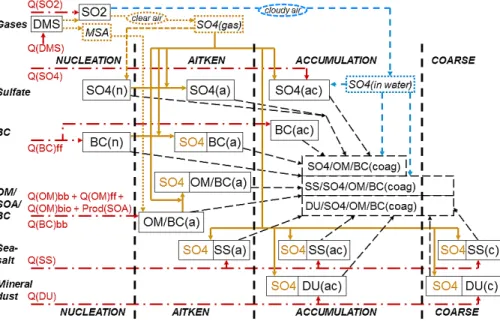
coagulation. The chemical components are sulphate (SO₄), black carbon (BC),

or-ganic matter (OM), sea-salt (SS), and mineral dust (DU). This adds up to 20 aerosol

components in addition to two gaseous precursors (SO₂and dimethyl sulphide, DMS).

Figure 1 gives an updated schematic representation of the aerosol processes in CAM4-Oslo.

5

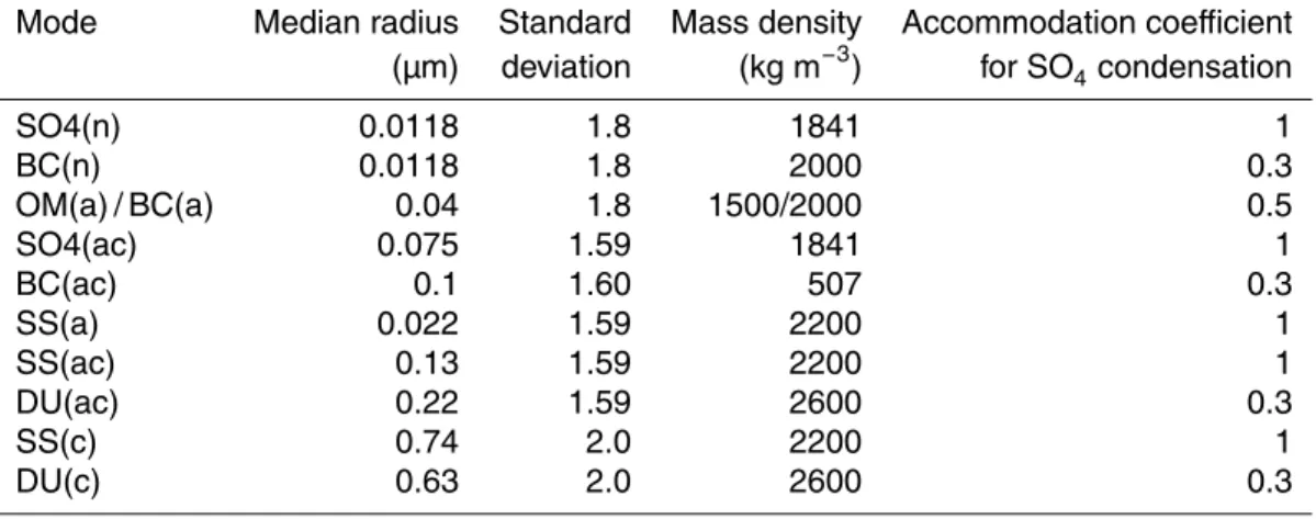
The basis for estimating particle numbers and sizes is assumptions made for the emitted or produced primary particles, of which there are 10 modes with log-normal size distributions as detailed in Table 1. These modes are changed in accordance with the processes to which the aerosol mass concentrations are tagged, and thus described without assuming log-normality using 44 size-bins with equal width with

re-10

spect to the logarithm of the particle radius. Hygroscopic swelling is calculated with the K ¨ohler equation. Optical properties are finally estimated from Mie-theory whilst CCN-activation is estimated based on super-saturation calculated from K ¨ohler theory (Abdul-Razzak and Ghan, 2000).

This chain of processes is, however, not calculated directly during integration of

15

NorESM or CAM4-Oslo. The optical and physical properties of the aerosols are in-stead estimated by interpolating between pre-calculated values in look-up tables. The process-tagged aerosol mass concentrations are given as input to the tables together with relative humidity. Output from one set of tables are dry aerosol modal radii and standard deviations based on log-normal fits to the size distributions, and are used for

20

estimating CCN-activation (Hoose et al., 2009). From a second set of look-up tables, spectrally resolved mass specific extinction, single scattering albedo, and asymmetry factor are used to estimate the influence of aerosols on short-wave radiation. The ta-bles are thoroughly described in Sect. 2.8 in Seland et al. (2008), see also Kirkev ˚ag and Iversen (2002).

25

(11)

GMDD

5, 2599–2685, 2012

Title Page

Tables Figures

◭ ◮

Back Close

Full Screen / Esc

Discussion

P

a

per

|

Dis

cussion

P

a

per

|

Discussion

P

a

per

|

Discussio

n

P

a

per

form SO₄(n) mode particles, with size parameters as given in Table 1. All particles are subject to condensation deposition of gaseous sulphate with an assumed accommoda-tion coefficient given in Table 1. Particles that are inefficient cloud condensation nuclei (such as pure BC and dust) may be transformed to become hydrophilic as they be-come internally mixed or coated by sulphate. Neither MSA (methane sulphonic acid),

5

biogenic OM, nor natural secondary organic aerosols (SOA) are separate variables, but are approximated to have the same properties as other OM compounds.

Aerosol components dissolved in cloud water are not kept as separate tracked vari-ables but are either scavenged or added to the general concentrations in air. The sul-phate produced by oxidation in cloud water droplets is thus distributed on accumulation

10

mode sulphate and on accumulation and coarse mode particles in internal mixtures re-sulting from coagulation in clear and cloudy air. This coagulation depletes the number of nucleation and Aitken mode particles by increasing the mass, but not the number, of accumulation and coarse mode particles. Details concerning gaseous and aqueous sulphur chemistry, the processes of nucleation, condensation, and coagulation, and

15

calculations of wet scavenging and dry deposition are given in Sect. 2.3 and Table 1 in Iversen and Seland (2002, 2003) with extensions in Sects. 2.3 through 2.8 in Seland et al. (2008). Some parameter values are changed in the present paper and also fitted to the new components not included in Seland et al. (2008). These are described in the next sub-sections.

20

2.1.1 Emissions of aerosols and aerosol precursors

Aerosol and aerosol precursor emissions have been updated. As indicated in Fig. 1,

emissions of 11 components are required (DMS, SO₂, SO₄, fossil fuel and biomass

burning BC and OM, biogenic OM and SOA production, sea-salt, and mineral dust). Several of these components can stem from both natural and anthropogenic sources

25

and represent preindustrial and present day stages in societal development.

(12)

GMDD

5, 2599–2685, 2012

Title Page

Tables Figures

◭ ◮

Back Close

Full Screen / Esc

Discussion

P

a

per

|

Dis

cussion

P

a

per

|

Discussion

P

a

per

|

Discussio

n

P

a

per

|

intercomparison excercise (e.g. Schulz et al., 2006, see also the official AeroCom web pages at http://aerocom.met.no) with emission data from Dentener et al. (2006). The new PI and PD emission years are taken as year 1850 and 2000 for CMIP5 simulations, and year 1850 and 2006 for use in the Phase II extension of AeroCom (Schulz et al., 2009; Ko_ffiet al., 2012b; Myhre et al., 2012; Samset et al., 2012). The emission years

5

1850 for PI and 2006 for PD are used as the standard in this paper, but test simulations with 1750 and 2000 emissions are also performed.

All simulations for years 1850 and 2000 employ emissions of SO₂, primary OM

(POM) and BC from fossil-fuel and bio-fuel combustion and biomass burning, as well as explicit BC emissions from aviation for year 2000, taken from the IPCC AR5 data

10

sets (Lamarque et al., 2010; Smith et al., 2011; Van der Werf et al., 2006; Schultz et al., 2008; Mieville et al., 2010; Buhaug et al., 2009; Eyring et al., 2009; Lee et al., 2009).

In the 2006 simulations the emissions for year 2000 are replaced by the Aerocom

Phase II emissions dataset. This dataset also includes emissions estimates of BC, SO₂

and POM from aviation. Since the IPCC AR5 year 2000 emissions of biomass burning

15

aerosols are 2D fields, we have assumed that these emissions have the same vertical profile as in the former Phase I of AeroCom, which was used in Seland et al. (2008).

An important part of the updated aerosol treatment in CAM4-Oslo is the treatment of natural background aerosols. These are particularly important for assessing the magni-tude of the indirect e_ffect of aerosols (see e.g. Kirkev ˚ag et al., 2008; Hoose et al., 2009;

20

Iversen et al., 2010), as well as for estimates of the total aerosol optical depth and

ab-sorption. Emissions of biogenic DMS, SO₂ from tropospheric volcanos, and mineral

dust are unchanged from Seland et al. (2008). The following two sub-sections present more details about new treatments of natural emissions of SOA from vegetation, bio-genic organic particles from oceans (Spracklen et al., 2008), and the temperature and

25

(13)

GMDD

5, 2599–2685, 2012

Title Page

Tables Figures

◭ ◮

Back Close

Full Screen / Esc

Discussion

P

a

per

|

Dis

cussion

P

a

per

|

Discussion

P

a

per

|

Discussio

n

P

a

per

2.1.2 Production of natural biogenic OM, SOA and MSA

Production of natural SOA from biogenic processes in land vegetation is taken into account as yield rates from terpene emissions and treated as emissions of POM. This is the same treatment as in Seland et al. (2008), but the total global emissions have been increased from 19.1 Tg yr−1 to 37.5 Tg yr−1. This is the production rate of natural

5

SOA minus a natural isoprene contribution estimated by Hoyle et al. (2007) in a model experiment where semi-volatile species were not allowed to partition to ammonium sulphate aerosol. Even larger production rates were found when this partitioning was allowed. Tsigaridis and Kanakidou (2003) suggested that the biogenic SOA production

from volatile organic compounds (VOC) may range from 2.5 to as much as 44.5 Tg yr−1.

10

Due to insufficient quantitative information about the sources, biogenic oceanic OM

is usually neglected in global climate models, even though it potentially contributes sig-nificantly to total OM (Matthias-Maser and Jaenicke, 1995; Bigg et al., 2004; Cavalli et al., 2004; O’Dowd et al., 2004; Jaenicke, 2005; Meskhidze et al., 2011; Despr ´es et al., 2012). Sources of this aerosol are thought to be primary emissions (POM) of

organic-15

enriched sea-spray aerosol from bubble bursting, and SOA formation from gas phase VOC emitted from the ocean surface (Facchini et al., 2008; Spracklen et al., 2008). In CAM4-Oslo we have included such a bio-aerosol in a simplified way and treated it as POM. Since data for the spatial and temporal distribution of the organic content in sea-water are not available on global scale, these biogenic OM emissions have, as a

20

first approximation, been given the same spatial distribution as the prescribed

Aero-Com fine mode sea-salt emissions. The global total of 8 Tg yr−1is based on Spracklen

et al. (2008). For comparison, the fossil fuel OM emission sources for 2006 amount to 6.3 Tg yr−1.

MSA, an oxidation product from DMS, was in Seland et al. (2008) assumed to be

25

(14)

GMDD

5, 2599–2685, 2012

Title Page

Tables Figures

◭ ◮

Back Close

Full Screen / Esc

Discussion

P

a

per

|

Dis

cussion

P

a

per

|

Discussion

P

a

per

|

Discussio

n

P

a

per

|

OM with an OM to S (Sulphur) mass ratio that is assumed to be the same as that of MSA to S (3.0).

Like the other OM emissions, both the two new contributions to oceanic OM de-scribed above are assumed to be emitted in the hydrophilic OM / BC Aitken mode; see Fig. 1.

5

2.1.3 Sea-salt emissions

A major upgrade in the natural aerosol treatment from the model version of Seland et al. (2008) is the replacement of the prescribed sea-salt emissions with prognostic sea-salt emissions based on Struthers et al. (2011). These emissions depend on 10-m

wind speed (U₁₀) and sea surface temperature (SST) (M ˚artensson et al., 2003), and

10

are regulated by the sea-ice cover as in Nilsson et al. (2001). The number flux (fluxn)

of each of the three log-normal sea-salt modes (Seland et al., 2008) at the point of emission, before hygroscopic growth and aerosol processing, have been fitted to the M ˚artensson et al. (2003) parameterization by using a quadratic function of SST:

fluxn=W ·(An·SST2+Bn·SST+Cn). (1)

15

This gives a simplified modal sea spray emission parameterization, compared to the detailed size distribution by M ˚artensson et al. (2003), that still preserves most of the wind and temperature dependency found in the original parameterization. The wind dependence, through the white cap fraction,

W ₌0.000384·U3.41

10 , (2)

20

is unchanged from Struthers et al. (2011). However, due to a simplified fitting of the coarse salt mode to the M ˚artensson et al. (2003) parameterization, tropical sea-salt burdens were somewhat exaggerated in Struthers et al. (2011). The SST depen-dence in the accumulation (SS(ac)) and coarse (SS(c)) modes in Table 1 of Struthers et al. (2011) has therefore been updated to improve the fit for particles with diameters

(15)

GMDD

5, 2599–2685, 2012

Title Page

Tables Figures

◭ ◮

Back Close

Full Screen / Esc

Discussion

P

a

per

|

Dis

cussion

P

a

per

|

Discussion

P

a

per

|

Discussio

n

P

a

per

greater than 2.5 µm, where the source parameterization of Monahan et al. (1986) is recommended. The revised coe_fficients are listed in Table 2.

2.1.4 Mass ratio OM / OC for biomass burning organic matter

We have increased the assumed mass ratio of particulate organic matter (OM) to or-ganic carbon (OC) for biomass burning emissions from 1.4 to 2.6. This number is taken

5

from Formenti et al. (2003) and is also used by Myhre et al. (2009). It leads to signif-icantly improved aerosol optical depths and absorption optical depths compared to observations and sun photometry retrievals in biomass burning dominated areas (see Sect. 5). The OM to OC mass ratio for SOA and for emissions from fossil fuel combus-tion is kept at 1.4, as in Seland et al. (2008).

10

2.1.5 Transport and removal in convective clouds

In the original CAM4 from NCAR, the convective cloud-cover is calculated explicitly. Hence, the volume available for convective scavenging is available directly. This is also the same formulation as in the chemistry transport model Mozart (Barth et al., 2000). Comparing CAM4 with CAM3, which was the host model of CAM-Oslo (used by Seland

15

et al., 2008), changes have been made to the deep convection scheme by including the

e_ffects of deep convection in the momentum equation and using a dilute approximation

in the plume calculation, which permits detrainment at all levels as opposed to only at the cloud top. These changes gave an improved representation of deep convection that occurs considerably less frequently but with higher intensity in CAM4 than in CAM3

20

(Gent et al., 2011). Based on the improved formulation of clouds with the dilute plume approximation (DPA) in CAM4, and on the resulting sulphate vertical distributions near the ITCZ, which are comparable to Seland et al. (2008), the special adjustment for aerosol processes in convective clouds (described in detail in Sect. 2.7 in Seland et al., 2008, see also Iversen and Seland, 2004), has been removed in CAM4-Oslo. We have

25

(16)

GMDD

5, 2599–2685, 2012

Title Page

Tables Figures

◭ ◮

Back Close

Full Screen / Esc

Discussion

P

a

per

|

Dis

cussion

P

a

per

|

Discussion

P

a

per

|

Discussio

n

P

a

per

|

convective cloud updrafts and downdrafts. A more realistic description should reflect the mixing generated by the horizontal shear between updrafts and downdrafts and the vigorous turbulence inside deep convective clouds. Assuming full mixing is a rad-ical assumption resulting in a minimum vertrad-ical transport of boundary-layer aerosols. Combined with the increased e_fficiency of scavenging by convective precipitation,

sys-5

tematically under-estimated aerosol burdens are likely to result. On the other hand, the choice we have made for CAM4-Oslo is prone to contribute to over-estimates. This is more thoroughly discussed in Sects. 4 and 5.

2.1.6 Oxidant chemistry

As in CAM-Oslo, tropospheric oxidant fields (OH, O₃, H₂O₂) for use in the sulphate

10

chemistry and the aerosol life cycle model are taken from simulations with a Chemical Transport Model (CTM). We have replaced the oxidant fields in Seland et al. (2008) with data from the most recent version of the oxidant chemistry in Oslo-CTM2 (Berntsen et al., 1997). H₂O₂is thus generally more abundant in lower tropospheric layers in CAM4-Oslo than in the version of Seland et al. (2008). Zonally and annually averaged, the

15

new H₂O₂ values are smaller in the upper troposphere (above about 500 hPa), much

smaller in the stratosphere, but larger in most of the lower troposphere, amounting to an increase by a factor larger than 2 in parts of the tropics.

Furthermore, the H₂O₂ replenishment time in cloudy air has been changed from a

fixed 1 h value (Seland et al., 2008) to a 1–12 h range, depending on the cloud

frac-20

tion. Within this 1–12 h range the replenishment time is assumed proportional to (1.1– c_max)−2_{, where}_c

maxis the maximum cloud fraction in the atmospheric column. This is

to account for the increase in time required for mixing larger volumes of air. The effect of this increased replenishment time would be opposite to the increased levels of H₂O₂ in the lower troposphere.

(17)

GMDD

5, 2599–2685, 2012

Title Page

Tables Figures

◭ ◮

Back Close

Full Screen / Esc

Discussion

P

a

per

|

Dis

cussion

P

a

per

|

Discussion

P

a

per

|

Discussio

n

P

a

per

2.1.7 Scavenging of mineral dust and gravitational settling

Modeled near surface mineral concentrations were underestimated approximately by a factor 2 in Seland et al. (2008). This negative bias may to some extent have been caused by missing mineral dust emissions, since the only source included in the emis-sion data set is major desert areas. On the other hand, the in-cloud scavenging

co-5

efficient for mineral dust was probably on the high side, since the assumed value of

1.0 implies that all mineral particles regardless of size or composition can be activated to form cloud droplets. In Hoose et al. (2009) the in-cloud scavenging coefficient for mineral dust was reduced to 0.1, leading to considerably extended residence times for mineral dust. In CAM4-Oslo, where the same mineral dust emissions are applied as in

10

the two previous studies, we use an intermediate in-cloud mineral scavenging coeffi

-cient value of 0.25, in agreement with the dominance of insoluble material. This yields about 25 % wet deposition globally averaged (Table 3), close to the median value of 28 % for 15 AeroCom Phase I models in a study by Huneeus et al. (2011). The individ-ual model averages in that work range from 16 % to 66 %.

15

Gravitational settling, which predominantly influences the largest particles, is now extended to all atmospheric levels in CAM4-Oslo, rather than in the lowermost level only (Seland et al., 2008). This is calculated at all heights, starting from the top of the model and calculating the contribution from each level to the model levels below. As a result the simulated aerosol removal is more e_fficient in general, particularly for coarse

20

mode aerosols.

2.2 Cloud droplet spectral dispersion

In Seland et al. (2008) a diagnostic relation between the aerosols and the liquid cloud droplet number (CDNC) was used for stratiform clouds, while liquid water content (LWC) was a prognostic variable (Rasch and Kristj ´ansson, 1998). A preliminary

sen-25

(18)

GMDD

5, 2599–2685, 2012

Title Page

Tables Figures

◭ ◮

Back Close

Full Screen / Esc

Discussion

P

a

per

|

Dis

cussion

P

a

per

|

Discussion

P

a

per

|

Discussio

n

P

a

per

|

forcing (the radius effect) by 36 % due to compensating effects not accounted for in the diagnostic scheme. The corresponding reduction in the joint first and second indirect forcing was estimated to 38 % in Kirkev ˚ag et al. (2008), using the same model version. The prognostic double moment cloud microphysics scheme has later become standard for stratiform clouds in the model (Storelvmo et al., 2006, 2008; Hoose et al., 2009).

5

As described by Hoose et al. (2009), calculation of realized supersaturation uses the sub-grid updraft velocity following Morrison and Gettelman (2008) and employs look-up tables for aerosol particle modal radii and standard deviations in the calculation of

activated CCN concentrations, used in subsequent calculations of CDNC and e_ffective

(with respect to scattering of light) cloud droplet radii (r_e_ff). For convective clouds these

10

quantities are estimated by simply assuming a supersaturation of twice the value for stratiform clouds.

A novelty compared to Hoose et al. (2009) is the introduction of a parameterization of cloud droplet spectral dispersion, allowing the shape of the cloud droplet spectrum to vary with changing aerosol loading.

15

The new formulation for cloud droplet spectral dispersion in CAM4-Oslo is taken from Eq. (2) in Rotstayn and Liu (2009), where the spectral shape factorβ (β≡r_e_ff/r_v;r_v

being the mean volume radius) is expressed as a monotonically increasing function of CDNC:

β₌

1₊2ε2

1+ε21/3 2_/3

, (3)

20

where the relative dispersionεis given by

ε₌1−0.7 exp(−0.003·CDNC·cm3). (4)

In both CAM4 (Neale et al., 2010) and CAM-Oslo (Kirkev ˚ag et al., 2008; Seland et al.,

2008; Hoose et al., 2009; Struthers et al., 2011), β was prescribed to values of 1.08

over oceans and 1.14 over land, independent of CDNC, following Martin et al. (1994).

(19)

GMDD

5, 2599–2685, 2012

Title Page

Tables Figures

◭ ◮

Back Close

Full Screen / Esc

Discussion

P

a

per

|

Dis

cussion

P

a

per

|

Discussion

P

a

per

|

Discussio

n

P

a

per

With the new treatment of Rotstayn and Liu (2009), we obtain largerβvalues for higher

levels of particle pollution. The new β is always larger than about 1.085. Thus β is

now larger over the oceans, and also over land whenever CDNC exceeds about 45– 50 cm−3.

The first indirect e_ffect is determined by the relative change inr_e_ff (Twomey, 1991),

5

and since r_e_ff ₌ r_v×β, the end result of the new β formulation is expected to be a smaller IndRF. Using an empirical scheme for CDNC as a function of aerosol mass

concentrations, Rotstayn and Liu (2009) showed that this β formulation gave a 34 %

reduction in the magnitude of the indirect radiative forcing. In this work we find a sig-nificantly smaller sensitivity to theβformulation; see Sect. 5. A recent survey of cloud

10

microphysical data from five field experiments by Brenguier et al. (2011) casts a new light on the issue of cloud droplet dispersion, but we have not attempted to include the results of that study here.

2.3 Parameter tuning

CAM4-Oslo applies the standard configuration of NCAR CAM4 with respect to model

15

physics, i.e. the Rasch and Kristj ´ansson (1998) scheme for stratiform cloud micro-physics and the CAM-RT radiation scheme (Collins et al., 2006), which were also used by both Seland et al. (2008) and Hoose et al. (2009). In order to obtain a realistic NorESM model climate while maintaining a net radiative balance at top of the atmo-sphere (TOA), some of the cloud micro- and macro-physical parameters have been

20

adjusted (Bentsen et al., 2012; Iversen et al., 2012) compared to the values used in CAM4. The minimum threshold for relative humidity in a model grid-cell for formation of low clouds, rhminl, has been reduced from 91 to 90 %. The critical mean droplet volume radius for onset of auto-conversion, denotedr_3lcin Rasch and Kristj ´ansson (1998), has been increased from 10 µm (Kristj ´ansson, 2002) to 14 µm. The value 15 µm was used

25

in Collins et al. (2006) and Seland et al. (2008). Furthermore, following Kristj ´ansson (2002), the precipitation rate threshold for suppression of auto-conversion of cloud

(20)

GMDD

5, 2599–2685, 2012

Title Page

Tables Figures

◭ ◮

Back Close

Full Screen / Esc

Discussion

P

a

per

|

Dis

cussion

P

a

per

|

Discussion

P

a

per

|

Discussio

n

P

a

per

|

used by e.g. Seland et al. (2008) and Hoose et al. (2009). Impacts of these changes on modelled aerosol properties, direct radiative forcing (DRF), cloud droplet number concentrations (CDNC), effective droplet radii (r_e_ff), liquid water path (LWP), and the indirect radiative forcing of aerosols (IndRF) are discussed in Sect. 5.

3 Model configuration and experiment set-up

5

For this study, CAM4-Oslo/NorESM has been set up to use the data ocean and

sea-ice models from CCSM4, running a series of 7-yroff-line simulations with IPCC AR5

or AeroCom aerosol and precursor emissions, see Sect. 2.1.1. TheCtrl simulations

(standard model version with all processes updated) are labelled PI and PD in Tables 3 through 7, where PI corresponds to aerosol emissions for year 1850 (“preindustrial”)

10

and PD corresponds to aerosol emissions for the year 2006 (“present day”). All sim-ulations use “present day” (year 2006) concentrations of greenhouse gases (GHG).

Running the model in an off-line mode means, in this case, that the meteorology is

driven by prescribed aerosol and cloud droplet properties of the standard CAM4 (but with CAM4-Oslo stratiform cloud tuning) in all the experiments. Hence, the meteorology

15

is the same in all simulations, except for a single sensitivity experiment where some of the tuning parameters for stratiform clouds have been changed. Calculation of the sec-ond indirect effect as a radiative forcing is as described by Kristj ´ansson (2002), i.e. by use of parallel calls to the condensation scheme as well as the scheme for radiative transport in the model.

20

The anthropogenic direct (DRF) and indirect forcing (IndRF) by aerosols since 1850

are found from the difference in net radiation energy fluxes between PD and PI. Our

results are based on the last 5 simulated years, except for the separate sensitivity test runs defined in Sect. 5 (Tables 5–7): here we instead show results from year 7 after a restart of the model from February year 6. All results are for short wave fluxes

25

(21)

GMDD

5, 2599–2685, 2012

Title Page

Tables Figures

◭ ◮

Back Close

Full Screen / Esc

Discussion

P

a

per

|

Dis

cussion

P

a

per

|

Discussion

P

a

per

|

Discussio

n

P

a

per

aerosols are allowed to affect the meteorology through their direct, semi-direct, and

indirect e_ffects on the radiation budget.

3.1 Sensitivity experiments

Each of the sensitivity experiments discussed in Sect. 5 is constructed by reverting each (or parts of each) of the model updates described in Sect. 2, back to the original

5

treatment in Seland et al. (2008), Hoose et al. (2009), or Struthers et al. (2011). In this way we are able to assess how much each of the updates has improved or changed

the model results, and to better understand differences in model behaviour between

CAM4-Oslo and other global models.

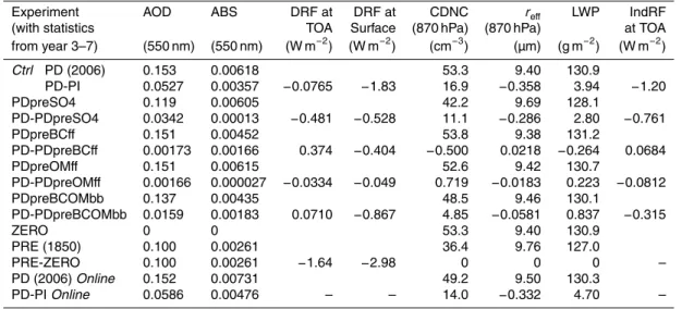
The additional simulations listed in Table 4 are forcing experiments originally set up

10

for estimating DRF for separate aerosol species (Myhre et al., 2012; Samset et al., 2012). However, in this paper also IndRF and relevant diagnostics for cloud droplet properties and cloud liquid water paths are examined. The only exception is the ZERO experiment. Here the aerosol extinction is set to 0 in the radiative transfer calculations, with no other changes. I.e. the aerosol life cycle and the cloud droplet properties are

15

as in theCtrl (PD) experiment, so that only optics and DRF are a_ffected.

4 Results

In order to validate the aerosol calculations in CAM4-Oslo and verify the results from the simulations labeledCtrl, we here discuss the aerosol concentrations, burdens,

life-times, optical properties, and effects on clouds and radiation in the model. We

com-20

pare calculated results with earlier model versions and with available observations or retrievals from remotely detected signals. Results of the sensitivity tests are discussed in Sect. 5.

Although not formally a part of the present study, more results from CAM4-Oslo as well as several other models, can be found at the AeroCom web-site:

(22)

GMDD

5, 2599–2685, 2012

Title Page

Tables Figures

◭ ◮

Back Close

Full Screen / Esc

Discussion

P

a

per

|

Dis

cussion

P

a

per

|

Discussion

P

a

per

|

Discussio

n

P

a

per

|

http://aerocom.met.no/data.html, where results labeled as CAM4-Oslo-Vcmip5 are

fromCtrl, CAM4-Oslo-Vcmip5online are from runs with on-line interactions with

me-teorological fields, and CAM4-Oslo-Vcmip5emi2000 are from runs with year 2000 as PD. The CAM-Oslo model version of Seland et al. (2008) is labeled UIO GCM V2.

4.1 Global aerosol budgets and atmospheric residence times

5

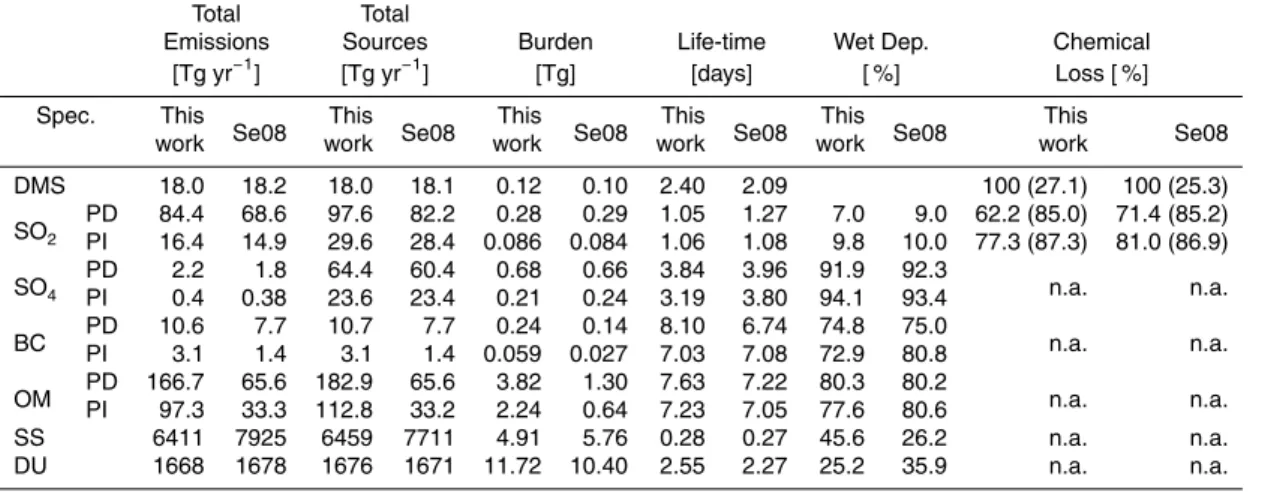
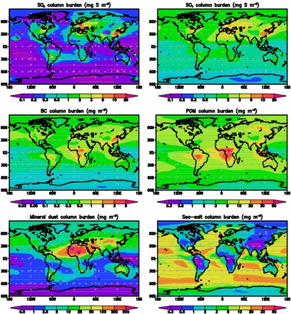
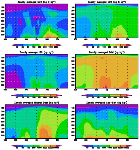
Table 3 compares the budgets and atmospheric residence times of CAM4-Oslo with the model-version presented by Seland et al. (2008). Figures 2 and 3 show maps of annual aerosol burdens and how the respective mass mixing ratios varies with height, zonally averaged.

For mineral dust, wet scavenging efficiency is reduced in CAM4-Oslo compared to

10

Seland et al. (2008), taking into account that mineral dust is not hygroscopic. This leads to a considerably reduced fraction of wet deposition of dust. Despite a more effective gravitational deposition due to the updated treatment of gravitational settling (see Table 6), we therefore find an increase in the global atmospheric burden and residence time (12 %).

15

The sea-salt burden is about 15 % lower than in Seland et al. (2008), in agreement with the smaller emissions (19 %). In spite of the enhanced importance of gravitational settling, the fraction deposited by precipitation scavenging is considerably higher in this work. This is probably a consequence of the wind (and SST) driven emissions in CAM4-Oslo. Strong winds over oceans are often co-located with precipitation. The

20

prescribed emissions in Seland et al. (2008) would more often, and erroneously, not be associated with the actual storms predicted in the atmospheric model, leaving a higher preference for dry rather than wet deposition.

Other major changes result from di_fferences in emission inventories when changing

from 2000 to 2006 for present day (PD) conditions and from 1750 to 1850 for

preindus-25

trial conditions (PI).

(23)

GMDD

5, 2599–2685, 2012

Title Page

Tables Figures

◭ ◮

Back Close

Full Screen / Esc

Discussion

P

a

per

|

Dis

cussion

P

a

per

|

Discussion

P

a

per

|

Discussio

n

P

a

per

close to values from many other models of the same type as CAM4-Oslo; see e.g. Tex-tor et al. (2006). For sulphate there is a considerable decrease for preindustrial condi-tions while for present day condicondi-tions there is a much smaller decrease. For OM and BC changes are relatively minor for preindustrial conditions, while there is an increase in residence time for the present day. The increase is particularly large for BC. For the

5

difference (PD-PI) an increase in atmospheric residence times is thus evident for all

the three aerosol components, but it is considerably larger for BC than for OM and sulphate. Since removal of these components to a large extent is determined by pre-cipitation scavenging, and their residence times are much too short for the components to reach a well-mixed state, changes in the geographical distribution of major emission

10

sources influence the residence time. This is in addition to changes in the e_fficiency of dry and wet removal processes.

If cloud volume and liquid water abundance were approximately the same as in Se-land et al. (2008), the increased levels of lower tropospheric H₂O₂ would tend to

re-duce the lifetime of both SO₂ and sulphate, by increasing the low-level oxidation and

15

producing sulphate in layers exposed to wet scavenging. Even though slightly reduced lifetimes are indeed calculated (Table 3), the reduction is counteracted by the slower replenishment of H₂O₂ in cloudy air and the more e_fficient vertical transport in deep convective clouds which brings low level air up to the middle and upper troposphere when mixing between downdrafts and updrafts is neglected. Furthermore, low-level

20

liquid water content and clouds are generally less abundant (a factor 60–80 % of the cloud cover in Seland et al., 2008) in CAM4-Oslo (not shown). It can also be noted from

Table 3 that the changes in wet scavenging and the overall fraction of SO₂oxidized in

(24)

GMDD

5, 2599–2685, 2012

Title Page

Tables Figures

◭ ◮

Back Close

Full Screen / Esc

Discussion

P

a

per

|

Dis

cussion

P

a

per

|

Discussion

P

a

per

|

Discussio

n

P

a

per

|

4.2 Comparison with measurements

4.2.1 Surface mass concentrations

Figure 4 compares modeled and measured near surface mass concentrations for each aerosol constituent. As described in more detail by Seland et al. (2008), the measure-ments span the years 1996–2002 and have been made available through the

Aero-5

Com project (http://aerocom.met.no) from the AEROCE, AIRMON, EMEP, GAW, and IMPROVE measurement networks. The EMEP data are from year 2002. Since results from a climate model are not designed to replicate single short-term observations but at best their overall statistics, monthly averaged data over the entire measurement

pe-riod are compared. The correlation coefficients and the fractions of modeled values

10

lying within a factor 2 and 10 of the measured values are listed in the figure legends.

With the relatively small scavenging coe_fficient compared to Seland et al. (2008),

we now get a 7 % positive bias in the average mineral dust concentration compared to the observed values in Fig. 4. This is a considerable improvement from the 55 % underestimate in Seland et al. (2008). Only 15 % of the modelled values were within

15

a factor of 2 of the measurements in Seland et al. (2008) whilst the corresponding percentage in this work is 44 %. The correlation coefficient is increased from 0.34 to 0.48. Ignoring the outliers for the highest concentrations in the upper right corner of the figure (sites close to the Sahara), there is still a negative bias in remote regions far from deserts. This may be an indication of missing sources, e.g. from semi-deserts

20

or smaller deserts which are not included in the model, agricultural regions, process industry, and road transport.

Although the sea-salt emissions are parameterized in a more physically based man-ner (temperature and wind dependency) than in Seland et al. (2008), where the emis-sions were simply prescribed, modeled near surface sea-salt mass concentrations in

25

(25)

GMDD

5, 2599–2685, 2012

Title Page

Tables Figures

◭ ◮

Back Close

Full Screen / Esc

Discussion

P

a

per

|

Dis

cussion

P

a

per

|

Discussion

P

a

per

|

Discussio

n

P

a

per

Seland et al. (2008). Overestimates are smaller for high concentrations than for lower concentrations. The prescribed emissions used in that work were pre-calculated val-ues (Dentener et al., 2006) with winds from a reanalysis of the meteorology for year 2000. Due to identical meteorology in all offline configurations of the present model set-up, the modeled sea-salt emissions are the same whether the anthropogenic emission

5

year is assumed to be 2000 or 2006. However, we do find considerable improvement in the sea-salt concentrations compared to the earlier version of the emission parame-terization used in Struthers et al. (2011); see Sect. 5.2.

Modeled SO₄concentrations are somewhat overestimated (23 %) and slightly more

so than in Seland et al. (2008), but with approximately the same correlation coefficient

10

(0.64) and percentage of modeled values within a factor of 2 of the measurements (77 %).

BC is underestimated with the same amount (18 %) as in Seland et al. (2008), but with a slightly lower correlation coe_fficient (0.43). One might suspect that this is a result

of using 2006 instead of 2000 BC emissions in theCtrl simulation. When we instead

15

use the 2000 emissions (theEmPD2000simulation, see Sect. 5.1), the correlation

co-e_fficient indeed improves (0.49), but the overall underestimate gets more severe (36 %). Also when comparing modeled AOD with ground and satellite based remote retrievals in Fig. 6, we get larger underestimates for most latitudes with the 2000 emissions. This is not caused by the di_fferences in BC emissions only.

20

OM concentrations are compared with measured OC concentrations in Fig. 4. The model does not keep track of the OM / OC ratio, resulting from the mixing of OM from

di_fferent sources. Thus OC in the present model version is not known. The comparison

with measured OC therefore requires an estimate of the (unknown) OM / OC mass ra-tio in the model. We should also keep in mind other potential sources of disagreement,

25

such as uncertain emission magnitudes, missing emission categories, and vertical mix-ing conditions.

(26)

GMDD

5, 2599–2685, 2012

Title Page

Tables Figures

◭ ◮

Back Close

Full Screen / Esc

Discussion

P

a

per

|

Dis

cussion

P

a

per

|

Discussion

P

a

per

|

Discussio

n

P

a

per

|

Sect. 2.1.4. Emissions of natural biogenic OM, SOA (treated as primary OM) and MSA are given directly as OM. Therefore the OM / OC ratios for these compounds are not required in the model itself. OM / OC ratios are typically somewhat larger than 1.4 for natural biogenic OM and SOA (e.g. Bergstr ¨om et al., 2012), and for MSA (CH₄O₃S) it is as large as 8.0. However, since MSA is not abundant over continents, its impact on

sur-5

face mass concentrations to be compared with observations are assumed small, except at coastal measurement sites. In Fig. 4 we have chosen to compare modeled OM / 1.4 with measured OC, assuming that OM / 1.4 is an upper estimate of the modeled OC concentration. These model values are thus representative for OC which mainly origi-nates from fossil fuel combustion sources, but are otherwise over-estimates.

10

For the North-American stations the modeled OM / 1.4 is 66 % larger than the mea-sured OC, while it was 9 % smaller in Seland et al. (2008). Here, 65 % of the data are within a factor of 2 of the measurements, and the correlation coefficient is 0.69. Hypo-thetically, assuming that all OM were from biomass burning, we should have compared OM / 2.6 with the measured OC values, yielding a 10 % negative bias. Splitting the data

15

in NH summer (April–September) and winter (October–March), marked in red and blue in Fig. 4, reveals that the correlation coe_fficient is about the same for both seasons, 0.69 and 0.68 respectively, but that the over-estimates are mostly confined to the

sum-mer (∼100 %) and that the modeled values of OM / 1.4 are very close to the observed

OC in winter (∼1 %). This may suggest that sources with OM / OC ratios which are

20

higher than 1.4 dominate in summer, or that OC concentrations are overestimated in summer.

However, the validation results for the European stations, using the OM / OC ratio of 1.4, suggest that modeled OM is still considerably underestimated in large regions.

The difference in model bias between European and North American stations is to

25

some extent caused by di_fferent measurement statistics. While the recommendation

for the North American OC measurements (IMPROVE, rural background stations) is to

use PM_2.5aerosol fraction, the European OC data (EMEP, including also some urban