Abs tract
In this paper, a mathematical model of large amplitude vibration of a uniform cantilever beam arising in the structural engineering is proposed. Two efficient and easy mathematical techniques called variational iteration method and He’s variational approach are used to solve the governing differential equation of motion. To assess the accuracy of solutions, we compare the results with the Runge-Kutta 4th order. An excellent agreement of the approxi-mate frequencies and periodic solutions with the numerical results and published results has been demonstrated. The results show that both methods can be easily extended to other nonlinear oscil-lations and it can be predicted that both methods can be found widely applicable in engineering and physics.
Key words
Large amplitude; Variational Iteration Method; He’s Variational Approach; Nonlinear oscillation.
Dynamic model of large amplitude vibration of a
uni-form cantilever beam carrying an intermediate lumped
mass and rotary inertia
1 INTRODUCTION
The Structural engineering theory is based upon physical laws and empirical knowledge of the
structural performance of different landscapes and materials. Many engineering structures can be
modelled as a slender, flexible cantilever beam carrying a lumped mass with rotary inertia at an
intermediate point along its span; hence they experience large-amplitude vibration (Wu, 2003;
Herisanu and Marinca, 2010; Cveticanin and Kovacic, 2007; Hamdan and Shabaneh, 1997; Hamdan
and Dado, 1997).
In general, such problems are not amenable to exact treatment and approximate techniques
must be resorted to. So, many new techniques have appeared in the open literature such as:
varia-tional iteration method (He, 2007a; Barari et al., 2011), homotopy perturbation method (Torabi
and Yaghoobi, 2011; Torabi et al., 2011; Saravi et al., 2013), homotopy analysis method (Liao,
2003; Khan et al., 2012)and some other methods (Nikkar et al., 2012; Ghasempoor et al., 2102;
Ak-barzade and Khan, 2012; Alinia et al., 2011; Ganji, 2012; Torabi et al., 2012; Sheikholeslami et al.,
A . N ik ka r *, 1, S. bag h eri1, M. S arav i2
1 Faculty of Civil Engineering, University of
Tabriz, Tabriz, Iran
2 Department of Mathematics, Islamic Azad
University, Nour Branch, Nour, Iran
Received in 19 Mar 2013 In revised form 30 Apr 2013
Latin American Journal of Solids and Structures 11(2014) 320 - 329
2012a; 2012b; Bayat et al., 2011; Rafieipour et al., 2012; Marinca and Herisanu, 2010; Salehi et al.,
2012; Hamidi et al., 2012)
The variational iteration method (VIM) and variational approach (VA) which were introduced
by He (He; 2007a;2007b) are very powerful methods in solving non-linear differential equations and
studying nonlinear vibration of beams. The Variational Approach which is also called He’s
varia-tional approach, as well as the variavaria-tional iteration method, was utilized here to obtain the
analyti-cal expression for the following model of nonlinear oscillations in the structural engineering
prob-lems:
0
)
(
2 3 22 2 2
2
=
+
+
+
+
u
dt
du
u
dt
u
d
u
u
dt
u
d
β
α
α
(1)
With initial conditions:
0
)
0
(
,
)
0
(
=
=
dt
du
A
u
(2)
This system describes the uni-modal large-amplitude free vibrations of a slender inextensible
cantilever beam carrying an intermediate mass with a rotary inertia. The third and fourth terms in
equation (1) represent inertia-type cubic non-linearity arising from the inextensibility assumption.
The last term is a static-type cubic nonlinearity associated with the potential energy stored in
bend-ing. The modal constants
α
and
β
result from the discretization procedure and they have specific
values for each mode as described in (Hamdan and Dado, 1997).
2 DESCRIPTION OF THE VARIATIONAL ITERATION METHOD
To clarify the basic ideas of proposed method consider the following general differential equation,
)
(
t
g
Nu
Lu
+
=
(3)
Where, L is a linear operator, and N a nonlinear operator, g(t) an inhomogeneous or forcing
term. According to the variational iteration method, we can construct a correct functional as
fol-lows:
τ
τ
τ
τ
λ
Lu
N
u
g
d
t
u
t
u
t
n n
n
n
(
)
(
)
(
(
)
~
(
)
(
)
)
0
1
=
+
∫
+
−
+
(4)
Where
λ
is a general Lagrange multiplier, which can be identified optimally via the variational
theory, the subscript n denotes the nth approximation,
u
~
nis considered as a restricted variation, i.e.
Latin American Journal of Solids and Structures 11(2014) 320 - 329
For linear problems, its exact solution can be obtained by only one iteration step due to the fact
that the Lagrange multiplier can be exactly identified. In this method, the problems are initially
approximated with possible unknowns and it can be applied in non-linear problems without
lineari-zation or small parameters. The approximate solutions obtained by the proposed method rapidly
converge to the exact solution.
3 IMPLEMENTATION OF VARIATIONAL ITERATION METHOD
Now, we can solve the following equation:
0
3 2 2=
+
+
+
+
u
u
u
u
u
u
u
α
α
β
(5)
with initial conditions:
0
)
0
(
,
)
0
(
=
A
u
=
u
(6)
Assume that the circular frequency of the system (5) is
ω
, we have the following linearized
equa-tion:
0
2=
+
u
u
ω
(7)
So we can rewrite Eq. (5) in the form:
0
)
(
2=
+
+
u
f
u
u
ω
(8)
Where
(
)
(
1
2)
2 2 30
=
+
+
+
−
=
u
u
u
u
u
u
u
f
ω
α
α
β
Applying the proposed method, the following iterative formula is formed as:
τ
τ
τ
ω
τ
λ
u
u
f
u
d
t
u
t
u
t
n n
n
n
(
)
(
)
(
(
)
(
)
(
(
)
)
02
1
=
+
∫
+
+
+
(9)
Its stationary conditions can be obtained as follows:
.
0
"
,
0
,
0
'
1
2
=
+
=
=
−
= =
=
t t
t
τ τ
τ
λ
ω
λ
λ
λ
(10)
The Lagrange multiplier, therefore, can be identified as;
)
(
sin
1
t
−
=
ω
τ
ω
Latin American Journal of Solids and Structures 11(2014) 320 - 329
Substituting the identified multiplier into Eq. (9) results in the following iteration formula:
τ
τ
β
τ
τ
α
τ
τ
α
τ
τ
τ
ω
ω
t
u
u
u
u
u
u
u
d
t
u
t
u
t n n n n n n n nn
sin
(
)(
(
)
(
)
(
)
(
)
(
)
(
)
(
)
)
1
)
(
)
(
0 3 2 21
=
+
∫
−
+
+
+
+
+
(12)
Assuming its initial approximate solution has the form:
)
cos(
)
(
0
t
A
t
u
=
ω
(13)
And substituting Eq. (13) into Eq. (5) leads to the following residual:
]
2
1
4
1
)[
3
cos(
)]
2
1
(
4
3
)[
cos(
)
(
cos
)
cos(
)
(
cos
2
)
cos(
)
cos(
)
(
2 3 3 3 2 3 3 3 2 3 3 2 3 2 0ω
α
β
ω
α
ω
β
ω
ω
β
ω
ω
α
ω
ω
α
ω
ω
ω
A
A
t
A
A
A
A
t
t
A
t
A
t
A
t
A
t
A
t
R
−
+
+
−
+
=
+
+
−
+
−
=
(14)
By the formulation (12), we can obtain
τ
τ
τ
ω
ω
t
R
d
t
u
t
u
t)
)
(
)(
(
sin
1
)
(
)
(
0 0 01
=
+
∫
−
(15)
In the same manner, the rest of the components of the iteration formula can be obtained. In order
to ensure that no secular terms appear in u
1, resonance must be avoided. To do so, the coefficient of
cos(
ω
t) in Eq. (14) requires being zero, i.e.,
4
2
4
3
2 2+
+
=
A
A
VIMα
β
ω
(16)
4 DESCRIPTION OF THE HE’S VARIATIONAL APPROACH
In 2007, the variational approach was proposed by He (He, 2007b). In this method, a variational
principle for the nonlinear oscillations is established, then a Hamiltonian is constructed, from which
the angular frequency can be obtained by a lacation method. To explain the method precisely,
con-sider the following generalized nonlinear oscillations without forced terms:
0
)
0
(
'
,
)
0
(
,
0
)
(
"
2=
=
=
+
+
u
f
u
u
A
u
u
ω
ε
(17)
where f is a nonlinear function of u, u ' and u".
Latin American Journal of Solids and Structures 11(2014) 320 - 329
dt
u
F
u
u
u
J
t
∫
⎭
⎬
⎫
⎩
⎨
⎧
+
+
−
=
0
2 2
)
(
2
2
'
)
(
ω
ε
(18)
where F is the potential, dF / du = f .
Its Hamiltonian reads
)
(
2
2
'
2u
2F
u
u
H
=
−
+
ω
+
ε
(19)
which should be an invariant during the oscillation. With the invariant, we can apply the location
method to identify the frequency by suitable choice of trial functions (He, 2006). If, by chance, the
exact solution had been chosen as the trial function, then it would be possible to make the residual
zero for all values of t by appropriate choice of
ω
. From this point of view, He’s variational method
is completely different from the classical variational methods, but has little likeness to Ritz method.
Because, Ritz method is only valid for fixed domain, but in He’s variational method, the integral
boundary is not fixed. So He’s functional formulation can be called as variational functional with
movable domain. Therefore, He’s variational approach is quite different from the classic Ritz
meth-od in calculus of variation. Following the approach adopted by the (Özi
ş
and Yildirim, 2006) in a
previous publication, He’s method has been used to determine the periodic solutions and the periods
of strongly nonlinear systems given below in subsequent three examples (Özi
ş
and Yildirim, 2006).
More recently, He’s method also adopted by D’Acunto for self-excited systems (D’Acunto, 2006a;
2006b).
5 IMPLEMENTATION OF HE’S VARIATIONAL APPROACH
The governing equation of the system is:
0
)
0
(
,
)
0
(
,
0
3 2 2=
=
=
+
+
+
+
u
u
u
u
u
u
u
A
u
u
α
α
β
(20)
We can, now, easily obtain the following variational formulation:
dt
u
u
u
u
u
u
J
T
∫
⎭
⎬
⎫
⎩
⎨
⎧
+
−
+
−
=
40
4 2 2 2
4
2
2
2
)
(
α
β
(21)
Assume that its approximate solution can be expressed as:
)
cos(
)
(
t
A
t
u
=
ω
(22)
Latin American Journal of Solids and Structures 11(2014) 320 - 329
).
8
1
64
3
32
8
(
)
(
2 2 2 2 2+
+
−
−
=
A
A
A
u
J
ω
α
ω
β
ω
π
(23)
Making J stationary with respect to A, according to He’s method (He, 2007b), we obtain:
0
)
32
3
16
(
)
8
1
64
3
32
8
(
2
2 2 2 2 2 2=
+
−
+
+
+
−
−
=
∂
∂
ω
β
ω
α
π
β
ω
α
ω
π
A
A
A
A
A
A
A
J
(24)
So the frequency can be approximated as:
4
2
4
3
2 2+
+
=
A
A
VAα
β
ω
(25)
and zero-order approximate solution from Eq.(22) is:
)
4
2
4
3
cos(
)
(
2 2t
A
A
A
t
u
+
+
=
α
β
(26)
6 RESULTS AND DISSCUSIONS
A mathematical model describing the process of large amplitude vibration of a uniform cantilever
beam arising in the structural engineering is proposed. Two different analytical methods are applied
to solve the dynamic model of the large amplitude non-linear oscillation equation. In order to verify
the precision of the methods, current results were compared with Runge-Kutta 4th order method in
Tables 1 and 2. It is observable that our results are in excellent agreement with the results provided
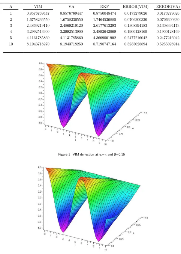
by Runge-Kutta 4th order. The behavior of
u
(
A
,
t
)
obtained by VIM and VA at
α
=
π
and
β
=0.15
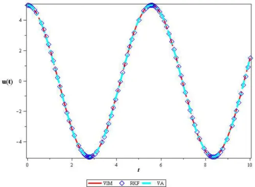
is shown in Figs. 1 and 2. The comparison of the displacement versus time for results obtained from
VIM, VA and Runge-Kutta 4th order has been depicted in Figs. 3 and 4 for
α
=
π
,
β
=0.15 and
A=5.
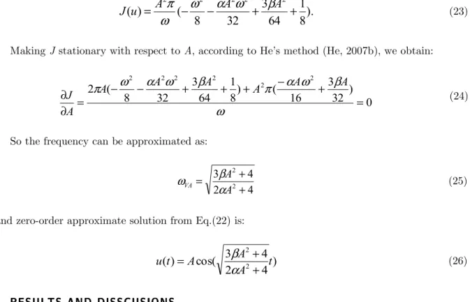
Table 1 Comparison between VIM & VA with time marching solution for the motion equation (5), when t = 0.5(s),
α=πandβ=0.15
Latin American Journal of Solids and Structures 11(2014) 320 - 329
Table 2 Comparison between VIM & VA with time marching solution for the motion equation (5), when t = 0.5(s), α= β=1
ERROR(VA) ERROR(VIM)
RKF VA
VIM A
0.0173279026 0.0173279026
0.8750048474 0.8576769447
0.8576769447 1
0.0706300330 0.0706300330
1.7464536880 1.6758236550
1.6758236550 2
0.1308394173 0.1308394183
2.6177613293 2.4869219120
2.4869219110 3
0.1900128169 0.1900128169
3.4892642069 3.2992513900
3.2992513900 4
0.2477216042 0.2477216042
4.3609001902 4.1131785860
4.1131785860 5
0.5255028914 0.5255028894
8.7198747164 8.1943718250
8.1943718270 10
Figure 2 VIM deflection at α=π and β=0.15
Latin American Journal of Solids and Structures 11(2014) 320 - 329 Figure 4 Comparison between VIM and VA periodic solutions versus time with Runge-Kutta 4th order for α=β=0.1 and A = 5.
Figure 5 Comparison between VIM and VA periodic solutions versus time with Runge-Kutta 4th order for α=β=0.1 and A = 5.
7 CONCLUSIONS
Latin American Journal of Solids and Structures 11(2014) 320 - 329
Results, it is shown that the approximate analytical solutions are in very good agreement with the
corresponding solutions.
References
Akbarzade, M., Khan, Y., (2012). Dynamic model of large amplitude non-linear oscillations arising in the struc-tural engineering: Analytical solutions. Mathematical and Computer Modelling, 55:480–489.
Alinia, M., Ganji, D. D., Gorji-Bandpy, M., (2011). Numerical study of mixed convection in an inclined two sid-ed lid driven cavity fillsid-ed with nanofluid using two-phase mixture model. International Communications in Heat and Mass Transfer, 38(10): 1428-1435.
Barari, A., Kaliji, H. D., Ghadimi, M., Domairry, G., (2011). Non-linear vibration of Euler-Bernoulli beams. Latin American Journal of Solids and Structures 8(2):139-148.
Bayat, Mahmoud., Pakar, Iman., Bayat, Mahdi., (2011). Analytical study on the vibration frequencies of ta-pered beams. Latin American Journal of Solids and Structures 8(2):149-162.
Cveticanin, L., Kovacic, I., (2007). Parametrically excited vibrations of an oscillator with strong cubic negative nonlinearity. Journal of Sound and Vibration, 304:201–212.
D’Acunto. M. (2006a). Self-exited systems: Analytical determination of limit cycles. Chaos, Solitons and Frac-tals, 30:719-724.
D’Acunto. M. (2006b). Determination of limit cycles for a modified van der Pol oscillator. Mechanics Research Communications 33:93-98.
Ganji, D. D. (2012). A semi-Analytical technique for non-linear settling particle equation of Motion. Journal of Hydro-environment Research 6(4): 323-327.
Ghasempour, S., Vahidi, J., Nikkar A., Mighani, M., (2012). Analytical Approach to Some Highly Nonlinear Equations by Means of the RVIM. Research Journal of Applied Sciences, Engineering and Technolo-gy, 5(1): 339-345.
Hamdan, M. N., Shabaneh, N. H., (1997). On the large amplitude free vibrations of a restrained uniform bean carrying an intermediate lumped mass. Journal of Sound and Vibration, 199:711–736.
Hamdan, M. N., Dado, M.H.F., (1997). Large amplitude free vibrations of a uniform cantilever beam carrying an intermediate lumped mass and rotary inertia. Journal of Sound and Vibration, 206:151–168.
Hamidi, S.M., Rostamiyan, Y., Ganji, D.D., Fereidoon, A., (2012). A novel and developed approximation for motion of a spherical solid particle in plane coquette fluid flow. Advanced Powder Technology, http://dx.doi.org/10.1016/j.apt.2012.07.00
He, J. H. (2006). Some asymptotic methods for strongly nonlinear equations. International Journal of modern Physics B, 20(10):1141-1199.
He, J.H., (2007a). Variational iteration method - some recent results and new interpretations. J Comput Appl Math, 20(1):3–17.
He, J. H. (2007b). Variational approach for nonlinear oscillators. Chaos, Solitons and Fractals, 34:1430–1439. He, J.H., (2012). Asymptotic methods for solitary solutions and compactions. Abstract and applied analysis, doi:10.1155/2012/916793
Herisanu, N., Marinca, V., (2010). Explicit analytical approximation to large-amplitude non-linear oscillations of a uniform cantilever beam carrying an intermediate lumped mass and rotary inertia. Meccanica, 45:847–855. Khan, Y., Taghipour, R., Fallahian, M., Nikkar, A., (2012). A new approach to modified regularized long wave equation. Neural Computing and Applications, doi:10.1007/s00521-012-1077-0
Latin American Journal of Solids and Structures 11(2014) 320 - 329
Marinca, V., Herisanu, N., (2010) Optimal homotopy perturbation method for strongly nonlinear differential equations. Nonlinear Science Letters A, 1(3): 273–280.
Nikkar, A., Mighani, Z., Saghebian, S.M., Nojabaei, S.B., Daie, M., (2012). Development and Validation of an Analytical Method to the Solution of Modelling the Pollution of a System of Lakes. Research Journal of Applied Sciences, Engineering and Technology, 5(1):296-302.
Öziş, T., Yildirim A., (2006). Determination of frequency-amplitude relation for Duffing-Harmonic oscillator by the energy balance method. Special Issue of Computers and Mathematics with Applications, 54(7):1184-1187. Rafieipour, H., Lotfavar, A., Mansoori, M.H., (2012). New Analytical Approach to Nonlinear Behavior Study of Asymmetrically LCBs on Nonlinear Elastic Foundation under Steady Axial and Thermal Loading. Latin Ameri-can Journal of Solids and Structures, 9(5):531-545.
Salehi, P., Yaghoobi, H., Torabi, M., (2012). Application of the Differential Transformation Method and Varia-tional Iteration Method to Large Deformation of Cantilever Beams under Point Load. Journal of Mechanical Science and Technology, 26 (9):2879-2887.
Saravi, M., Hermaan, M., Ebarahimi khah, H., (2013). The comparison of homotopy perturbation method with finite difference method for determination of maximum beam deflection. Journal of Theoretical and Applied Physics, 7:8, doi:10.1186/2251-7235-7-8
Sheikholeslami, M., Soleimani, S., Gorji-Bandpy, M., Ganji, D. D., Seyyedi, S. M., (2012a). Natural convection of nanofluids in an enclosure between a circular and a sinusoidal cylinder in the presence of magnetic field. International Communications in Heat and Mass Transfer, 39(9): 1435-1443.
Sheikholeslami, M., Gorji-Bandpy, M., Ganji, D. D., (2012b). Magnetic field effects on natural convection around a horizontal circular cylinder inside a square enclosure filled with nanofluid. International Communica-tions in Heat and Mass Transfer, 39(7): 978-986
Torabi, M., Yaghoobi, H., (2011). Novel Solution for Acceleration Motion of a Vertically Falling Spherical Particle by HPM-Pade Approximant. Advanced Powder Technology, 22:674-677.
Torabi, M., Yaghoobi, H., Saedodin, S., (2011). Assessment of Homotopy Perturbation Method in Nonlinear Convective-Radiative Non-Fourier Conduction Heat Transfer Equation with Variable Coefficient. Thermal Science, 15:263-274.