Abstract
Dynamic compression behaviors of density-homogeneous and densi-ty-graded irregular honeycombs are investigated using cell-based finite element models under a constant-velocity impact scenario. A method based on the cross-sectional engineering stress is developed to obtain the one-dimensional stress distribution along the loading direction in a cellular specimen. The cross-sectional engineering stress is contributed by two parts: the node-transitive stress and the contact-induced stress, which are caused by the nodal force and the contact of cell walls, respectively. It is found that the contact-induced stress is dominant for the significantly enhanced stress behind the shock front. The stress enhancement and the compac-tion wave propagacompac-tion can be observed through the stress distribu-tions in honeycombs under high-velocity compression. The single and double compaction wave modes are observed directly from the stress distributions. Theoretical analysis of the compaction wave propagation in the density-graded honeycombs based on the R-PH (rigid–plastic hardening) idealization is carried out and verified by the numerical simulations. It is found that stress distribution in cellular materials and the compaction wave propagation character-istics under dynamic compression can be approximately predicted by the R-PH shock model.
Keywords
dynamic crushing, density gradient, stress distribution, stress enhancement, shock wave speed
Stress Distribution in Graded Cellular
Materials Under Dynamic Compression
1 INTRODUCTION
Cellular materials have gained much research interest due to their significant capacity in impact energy absorption and blast attenuation (Gibson and Ashby 1997; Lu and Yu 2003). Their dynamic crushing behaviors have been studied extensively and much knowledge has been obtained. Stress enhancement and deformation localization are two typical characteristics of cellular materials under
Peng Wang a Xiaokai Wang a Zhijun Zheng a, * Jilin Yu a
a CAS Key Laboratory of Mechanical
Behavior and Design of Materials, Uni-versity of Science and Technology of China, Hefei, Anhui 230026, PR China
* Corresponding author: [email protected]
http://dx.doi.org/10.1590/1679-78253428
dynamic crushing. However, most research work is restricted to the stress at the impact/support end and thus the stress distribution is not well considered.
Significant enhancement of crushing stress was observed in the dynamic impact experiments of woods (Reid and Peng, 1997; Harrigan et al., 2005), aluminum honeycombs (Zhao and Gary, 1998; Hou et al., 2012) and foams (Mukai et al., 1999; Deshpand and Fleck, 2000; Tan et al., 2005a; Elnasri et al., 2007). Several shock models and mass-spring models have been proposed to under-stand the shock wave propagation in cellular materials under dynamic impact, such as the R-PP-L (rate-independent, rigid–perfectly plastic–locking) model (Reid and Peng, 1997), the mass-spring model (Li and Meng, 2002), the E-PP-R (elastic–perfectly plastic–rigid) model (Lopatnikov et al., 2003), the power law densification model (Pattofatto et al., 2007) and the D-R-PH (dynamic, rigid– plastic hardening) shock model (Zheng et al., 2014). Because the assurance of the repeatability of samples and the measurement of local stress and strain states have not been well solved by experi-mental techniques, finite element (FE) method has been applied to simulate the dynamic crushing of cellular materials, such as regular/irregular honeycombs (Ruan et al., 2003; Zheng et al., 2005; Liu et al., 2009; Zou et al., 2009; Hu and Yu, 2013) and open-/closed-cell foams (Gaitanaros and Kyriakides, 2014; Zheng et al., 2014; Sun et al., 2016). The typical features of stress enhancement and deformation localization can be appropriately represented.
un-derstand the shock wave propagation and stress enhancement. However, direct evidence, e.g. the local stress, is insufficient.
A method based on the optimal local deformation gradient was proposed by Liao et al. (2013) to calculate the local strain field of Voronoi honeycombs. The propagation of shock wave was found to be obviously one-dimensional no matter under the Shock Mode or the Transitional Mode. Zou et al. (2009) proposed a method based on nodal accelerations to obtain the stress distribution in hex-agonal-cell honeycombs numerically. However, it is an indirect method and the data oscillation is obvious especially when the impact velocity is high enough. Direct information about local stress is insufficient because the discussion about the dynamic stress in the literature is mostly focused on the proximal and distal ends no matter experimentally and numerically. Therefore, efforts have been made in this study to propose a method to calculate the cross-sectional stress and acquire the one-dimensional stress distribution along the cellular material, by which a better comprehension on the stress enhancement and shock wave propagation can be reached.
In this study, virtual tests of density-graded honeycombs under constant-velocity compression are carried out to understand the dynamic behavior of graded cellular materials. A cross-sectional stress calculation method is proposed to obtain the stress distribution of density-graded honeycombs under compression. Finally, comparisons of stress distributions obtained from the cross-sectional stress calculation method and one-dimensional shock models are made.
2 NUMERICAL SIMULATIONS AND STRESS CALCULATION METHOD
2.1 Cell-Based Finite Element Models
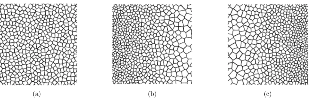
The 2D Voronoi technique is employed here to construct irregular honeycombs with a homogene-ous/graded density, see Refs. (Zheng et al., 2005) and (Wang et al., 2011) for details. The density-graded honeycombs are constructed by changing the cell size distribution in a specific manner but keeping the cell-wall thickness constant. The relative density distribution of graded honeycomb
specimens along the X-axis is considered to be linear, written as
f s 0
( )X ( ) /X 1 X /L1/ 2
, (1)where λ is the density-gradient parameter, L the length, ρf the local density, ρ0 the average relative
density of honeycomb specimens and ρs the density of matrix material. Three specimens of irregular
honeycombs with λ = 0, −1 and 1 are illustrated in Figure 1. The cell irregularity of specimens is
0.3 and the average relative density ρ0is 0.1. The length, width and thickness of specimens are 100
mm, 100 mm and 1 mm, respectively. The cell walls in a specimen have an identical thickness, which is about 0.23 mm in this study.
The FE code ABAQUS/Explicit is employed to perform virtual tests. The specimens are modeled with S4R elements. The matrix material of cell walls is assumed to be elastic, perfectly plastic with
Young’s modulus E = 66 GPa, Poisson’s ratio ν = 0.3, yield stress ys= 170 MPa, and density ρs =
2700 kg/m3. All nodes are constrained in the out-of-plane direction to simulate a plane strain situation.
constant velocity, V, to the right, i.e. along the X direction. In this study, the nodal force and con-tact force are obtained from the ABAQUS output files to calculate the cross-sectional stress.
(a) (b) (c)
Figure 1: Samples of honeycomb specimens with (a) λ = 0, (b) λ= −1 and (c) λ = 1.
2.2 Calculation of One-Dimensional Cross-Sectional Stress
In the cell-based FE models, meso-structural deformation and mechanical responses can be accu-rately represented. Information, such as the stress and strain of every element, can be obtained from the ABAQUS output files but it cannot be used to represent the local stress/strain at the continu-um level. Based on the optimal local deformation gradient technique, a local strain field calculation method for cellular materials has been developed by Liao et al. (2013, 2014) to calculate the local strain. However, the local stress cannot be calculated in a similar manner and the mission of calcu-lating the local stress field for cellular materials seems to be impossible. Fortunately, it was ob-served that the propagation of shock wave is in a nearly one-dimensional form when cellular materi-als are crushed under high-velocity impact (Reid and Peng, 1997; Ruan et al., 2003; Tan et al., 2005a; Zou et al., 2009; Liao et al., 2013) and the one-dimensional approximation is popularly used. Thus, we can focus on the one-dimensional stress distribution and use the force on the cross section of cellular material to calculate the cross-sectional stress.
(a) (b) (c)
Figure 2: Schematic diagrams of (a) a cross section in the reference configuration, (b) nodal
force without contact and (c) contact situation in the current configuration. Contact
In this study, the one-dimensional engineering stress is defined at a number of cross sections at different Lagrangian locations along the loading direction of a cellular specimen. Schematic dia-grams of a cross section in the reference configuration and force conditions with/without contact are shown in Figure 2. The investigated cross section is a Lagrangian one, which crosses a plenty of elements in the reference configuration, as diagrammed in Figure 2(a). When the deformation is small and cells are not in contact, the macroscopic stress transferring from the proximal end to the distal end is realized by the nodes, which connect the relevant elements. The components of the
nodal force of Node i are denoted as Fn xi and F
n
yi, see Figure 2(b). The nodal force can be extracted
directly from the output file of the FE simulation. Therefore, the cross-sectional internal force caused by the nodal force without contact can be calculated by
n n
1
M
x xi
i
F F
, (2)where M is the number of nodes at the left side of the elements crossed by the cross section in the
reference configuration. Then, the corresponding stress n
x, named as the node-transitive stress
here-after,is calculated by
n n
0
/
xx
F
A
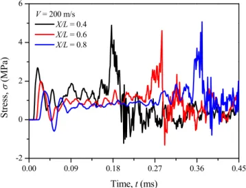
, (3)where A0 is the initial cross-sectional area of the cellular specimen. Figure 3 shows the variation of
the node-transitive stress with time at the impact velocity of 200 m/s. If there is no contact be-tween cell walls, the cross-sectional stress can be represented by the node-transitive stress.
0.00 0.09 0.18 0.27 0.36 0.45
-2 0 2 4 6
V = 200 m/s X/L = 0.4 X/L = 0.6 X/L = 0.8
Stress,
(MPa)
Time, t (ms)
Figure 3: History of the node-transitive stresses at different Lagrangian locations
for a homogeneous honeycomb at an impact velocity of 200 m/s.
However, it is difficult to track and judge the contact pairs locating on the specified cross section, because the generation of contact seems very random and the number of contact pairs increases greatly during the impact process. A lot of time and efforts will be spent on searching the relevant contact pairs of the investigated cross section. Fortunately, we can use another way, which is much simple and meaningful, to calculate the contact force on the cross section. According to the New-ton’s third law, the contact forces of a complete contact pair are equal in value and opposite in direction. In the FE simulation, the contact force of a contact pair is assigned to the associated nodes. Thus, the cross-sectional contact force can be obtained by the superposition of all contact forces of the cellular specimen on the left side of the cross section and those of the nodes belong to the impact plate. In this process, the contact forces of a complete contact pair cancel each other and the contact force on the cross section can be obtained. Hence, the contact force of the cross section,
denoted as Fcx, can be formulated as
c cn ct
1
N
x xi xi
i
F
F
F
, (4)where Fcnxi and F
ct
xi are the loading directional components of the normal contact force and tangential
contact force respectively obtained from the output file, and N is the number of the nodes on the
left side of the cross section. Similarly, the corresponding stress c
x induced by contact is determined
by
c c
0
/
xx
F
A
. (5)Hereafter, this stress is named as the contact-induced stress. Thus, the cross-sectional stress x
can be calculated by
n c
x
x
x
. (6)2.3 Feasibility Verification of the Cross-Sectional Stress Calculation Method
In the Quasi-static mode, the deformation shear bands occur randomly (Zheng et al., 2005; Liu et al., 2009). The force balance should be satisfied in the loading direction at the macro scale because the inertia effect can be ignored under quasi-static situation (Liu et al., 2009). Figure 4 shows that stress balance is almost satisfied at any three nominal strains for the equally distributed stress along the homogeneous honeycomb specimen at the impact velocity of 1 m/s. Therefore, the cross-sectional stress calculation method proposed in this study is applicable.
2.4 Comparison Between Node-Transitive Stress and Contact-Induced Stress
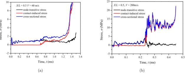
By applying the cross-sectional stress calculation method, the node-transitive, contact-induced and cross-sectional stresses for a homogeneous honeycomb under dynamic compression are analyzed. For
example, the stress history curves for a homogeneous honeycomb at the middle position X/L = 0.5
of the specimen. No contact occurs at the middle position which is far ahead of the shock front. After the shock front reaches the middle position, the node-transitive stress changes not much, but the contact-induced stress changes to a large value, which has the same variation tendency with the cross-sectional stress. This is because numerous cell walls contact in the compacted region behind the shock front.
0.0 0.2 0.4 0.6 0.8 1.0
0 1 2 3 4 5
St
re
ss,
(MPa)
Lagrangian position, X/L
N = 0.2 N = 0.5 N = 0.8
Figure 4: Stress distributions of a homogeneous honeycomb at three nominal strains at the impact velocity of 1 m/s.
0.0 0.2 0.4 0.6 0.8 1.0 1.2 1.4 1.6 -2
0 2 4 6 8 10
St
re
ss,
(MP
a)
Time, t (ms) node-transitive stress contact-induced stress cross-sectional stress X/L = 0.5 V = 60 m/s
0.0 0.1 0.2 0.3 0.4 0.5 -5
0 5 10 15 20 25
St
re
ss
,
(MPa)
Time, t (ms)
node-transitive stress contact-induced stress cross-sectional stress X/L = 0.5, V = 200m/s
(a) (b)
Figure 5: Variations of stresses at the middle position with time for a homogeneous
honeycomb at different impact velocities: (a) V = 60 m/s and (b) V = 200 m/s.
0.0 0.1 0.2 0.3 0.4 0.5 0
5 10 15 20
V = 200 m/s
X/L = 0.1 X/L = 0.2 X/L = 0.3 X/L = 0.4 X/L = 0.5
Averaged
Stress,
(M
Pa)
Time, t (ms)
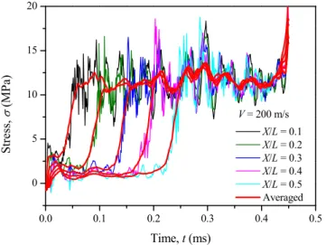
Figure 6: Variations of cross-sectional stress with impact time at different cross sections.
2.5 Relation Between Cross-Sectional Stress and Impact Time
The stress–time relation at different positions is presented in Figure 6. The curves have significant oscillation, especially at a very high impact velocity, e.g. 200 m/s. This is due to the contact algo-rithm of the FE analysis and the propagation of complex stress waves in the specimen. Liao et al. (2014) found that the local nature and accuracy of the strain field calculation method are strongly dependent on the cut-off radius, which is introduced to collect the effective nodes for determining the optimal local deformation gradient of a node. Through sensitivity analysis, the optimal cut-off radius defined based on the reference configuration was found to be about 1.5 times of the average cell radius (Liao et al., 2014). In order to exclude the influence of the data oscillation, Zheng et al. (2014) averaged the relation between the shock stress and impact time over a certain time interval. For better consistency with the local strain field method, the relation between cross-sectional stress and impact time is averaged herein over a time interval , which corresponds to the time when cells
in a width of a 1.5 times average cell size is crushed. The time interval is calculated by
0 s
1.5 /
d
V
, (7)where d0 is the average cell size and Vs the shock wave speed. For simplicity, the shock wave speed
is directly calculated from the R-PP-L shock model (Reid and Peng, 1997; Liao et al., 2013), i.e. Vs
= V/εL, where εL is the locking strain, which is defined as the strain when the maximum value of
3 RESULTS AND DISCUSSION
3.1 Deformation Patterns and Stress Distribution
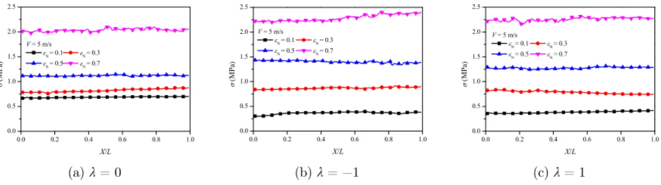
Three deformation modes have been observed in irregular honeycombs under dynamic compression (Zheng et al., 2005; Liu et al., 2009), i.e., Quasi-static Mode, Transitional Mode and Shock Mode. In this study, the cross-sectional stress calculation method provides a way to understand the stress distribution along the specimen and how the stress wave propagates. The one-dimensional stress distributions of homogeneous and density-graded honeycombs under constant-velocity compression together with deformation patterns are analyzed in this section.
0.0 0.2 0.4 0.6 0.8 1.0 0.0
0.5 1.0 1.5 2.0 2.5
V = 5 m/s
N = 0.1 N = 0.3
N = 0.5 N = 0.7
MPa
X/L
0.0 0.2 0.4 0.6 0.8 1.0 0.0
0.5 1.0 1.5 2.0 2.5
V = 5 m/s
N = 0.1 N = 0.3
N = 0.5 N = 0.7
MPa
X/L
0.0 0.2 0.4 0.6 0.8 1.0 0.0
0.5 1.0 1.5 2.0 2.5
V = 5 m/s N = 0.1 N = 0.3
N = 0.5 N = 0.7
MPa
X/L
(a) λ= 0 (b) λ= −1 (c) λ= 1
Figure 7: One-dimensional stress distributions of homogeneous and
density-graded honeycombs at an impact velocity of 5 m/s.
(a) λ= 0 (b) λ= −1 (c) λ= 1
Figure 8: Deformation patterns of homogeneous and density-graded
honeycombs at εN = 0.4 at an impact velocity of 5 m/s.
When the impact velocity is low (say, 5 m/s), for all the three density-graded parameters (λ =
0, −1 and 1) considered, the stress in the specimens is almost equally distributed. This indicates
that the specimen under low-velocity compression is in a state of force/stress equilibrium no matter
the density gradient is. With the increase of nominal strain N (i.e. the impact time), the stress
gradu-ally changes due to the density gradient, and thus the deformation occurs first at the position where the relative density is relatively less, see Figure 8(b) and (c). The deformation bands generate a compaction wave, which front propagates from the low density to the high density.
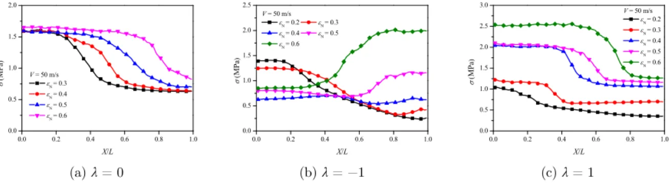
When the impact velocity is moderate (say, 50 m/s), the stress distributions show some
differ-ent features. For λ = 0, the location where the stress sharply changes moves to the support end
with the increase of impact time. This location represents a shock front. The stress behind the shock front keeps at the same level due to the constant density and impact velocity, as shown in Figure 9(a). However, for density-graded honeycombs, the stress distributions are very different
from those of homogeneous honeycombs. For λ < 0, evenly distributed stress appears near the two
ends of the specimen, varying with the increase of nominal strain, as shown in Figure 9(b). A dou-ble shock mode was employed to describe the deformation mode in which the deformation bands locate at the two ends of the negative-gradient specimen in Refs. (Shen et al., 2013; Wang et al., 2013; Shen et al., 2014). According to the stress distribution, the double shock mode is also ob-served in this study. The stresses behind and ahead of the shock front near the impact end decrease with the increase of nominal strain. This is because the local density at the shock front, which rep-resents the crash strength, decreases with the motion of shock front. Although the double shock mode has been reported in the literature, it should be noted that the deformation close to the sup-port end is very small and the deformation bands are random, and thus it is more appropriate to call the “shock wave” near the support end as a “compaction wave”. The stresses behind and ahead of the wave front near the support end increase with the increase of nominal strain due to the
nega-tive density gradient. For λ > 0, the stresses behind and ahead of the wave front increase with the
increase of nominal strain, see Figure 9(c). This is because the local density of the wave location
increases with the increase of nominal strain. The deformation of honeycombs with λ > 0 is more
localized than that of the homogeneous honeycombs, see Figure 10.
0.0 0.2 0.4 0.6 0.8 1.0 0.0
0.5 1.0 1.5 2.0
V = 50 m/s N = 0.3
N = 0.4
N = 0.5
N = 0.6
X/L
MPa
0.0 0.2 0.4 0.6 0.8 1.0 0.0 0.5 1.0 1.5 2.0 2.5
V = 50 m/s
N = 0.2 N = 0.3
N = 0.4 N = 0.5
N = 0.6
MPa
X/L
0.0 0.2 0.4 0.6 0.8 1.0 0.0 0.5 1.0 1.5 2.0 2.5 3.0
V = 50 m/s
N = 0.2
N = 0.3
N = 0.4
N = 0.5
N = 0.6
MPa
X/L
(a) λ= 0 (b) λ= −1 (c) λ= 1
Figure 9: One-dimensional stress distributions of homogeneous and
density-graded honeycombs at an impact velocity of 50 m/s.
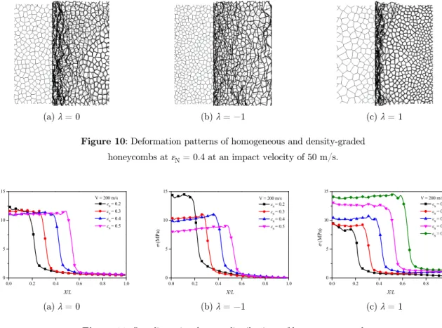
When the impact velocity is high enough (say, 200 m/s), a single shock wave front propagates to the right with the increase of nominal strain, see Figure 11, which can also be observed in the deformation patterns of the specimens in Figure 12. The deformation localizes near the impact end
regardless of the values of λ, but the levels of densification are different. The width of the
descend-ing order. The stress behind the shock front is significantly enhanced for the three kinds of
honey-combs, see the stress distributions in Figure 11. For λ = 0, the stress behind the shock front keeps
at the same level. For λ < 0, the stress behind the shock front decreases with the increase of
nomi-nal strain, but for λ > 0, it increases with the increase of nominal strain. These features are mainly
due to the density gradients.
(a) λ = 0 (b) λ = −1 (c) λ = 1
Figure 10: Deformation patterns of homogeneous and density-graded
honeycombs at εN = 0.4 at an impact velocity of 50 m/s.
0.0 0.2 0.4 0.6 0.8 1.0 0
5 10 15
V = 200 m/s
N = 0.2
N = 0.3
N = 0.4
N = 0.5
MPa
X/L
0.0 0.2 0.4 0.6 0.8 1.0 0
5 10 15
V = 200 m/s
N = 0.2
N = 0.3
N = 0.4
N = 0.5
MPa
X/L
0.0 0.2 0.4 0.6 0.8 1.0 0
5 10 15
V = 200 m/s
N = 0.2
N = 0.3
N = 0.4
N = 0.5
N = 0.6
MPa
X/L
(a) λ = 0 (b) λ = −1 (c) λ = 1
Figure 11: One-dimensional stress distributions of homogeneous and
density-graded honeycombs at an impact velocity of 200 m/s.
(a) λ = 0 (b) λ = −1 (c) λ = 1
Figure 12: Deformation patterns of homogeneous and density-graded
3.2 Comparison with Shock Model
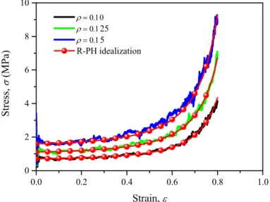
The propagation of shock wave has been described by the one-dimensional shock models in Refs. (Tan et al., 2005b; Li and Reid, 2006; Karagiozova et al. 2012). The quasi-static stress–strain curve for the uniform density material is shown in Figure 13. The R-PH idealization is employed to model the quasi-static stress–strain curve. Compared to the classical R-PP-L idealization, the R-PH ideali-zation is more appropriate to describe the mechanical behavior of cellular materials. Thus in this study, the R-PH shock model is applied to describe the shock propagation behavior of irregularly graded honeycombs under constant-velocity compression. The detailed derivations of the R-PH shock models are presented in Appendix A.
0.0 0.2 0.4 0.6 0.8 1.0
0 2 4 6 8 10
St
ress,
(M
Pa)
Strain,
25
5
R-PH idealization
Figure 13: The quasi-static stress–strain curve for the uniform density material.
In the R-PH idealization, the stress−strain relation is written as (Zheng et al., 2014)
20
( ) = +
C
/ 1
, (8)where 0 is the initial crush stress and C the strain hardening parameter, which can be obtained by
fitting the quasi-static stress−strain curves. The initial crush stress of cellular material is related to
the relative density of cellular material (Gibson and Ashby, 1997), written as
2 0
( )
/
ys
. (9)ys
( ) /
nC
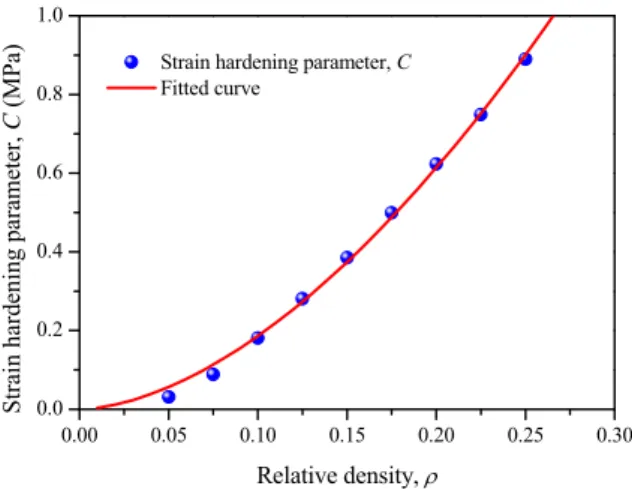
, (10)where the fitting parameters and n are determined as 0.0576 and 1.721, respectively, in this study.
The shock wave speed based on the R-PH shock model (Zheng et al., 2014) can be calculated as Vs
= V + c, where c C( ) /
s for a specified relative density of cellular material. Fordensity-graded honeycombs, the shock wave propagation is much more complex, see Appendix A.
0.00 0.05 0.10 0.15 0.20 0.25 0.30
0.0 0.2 0.4 0.6 0.8 1.0
Strain hardening parameter, C
Fitted curve
Strai
n ha
rdeni
ng pa
rame
te
r,
C
(MPa)
Relative density,
Figure 14: Variations of the strain hardening parameter with the relative density.
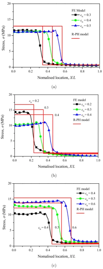
0.0 0.2 0.4 0.6 0.8 1.0 0
5 10 15 20
FE Model N = 0.3 N = 0.4 N = 0.5
St
re
ss
,
(MP
a)
Nomalised location, X/L
R-PH model
(a)
0.0 0.2 0.4 0.6 0.8 1.0
0 5 10 15 20
FE model
N = 0.2
N = 0.3
N = 0.4 R-PH model
Stress,
(MPa)
Nomalised location, X/L N = 0.2
0.3
0.4
(b)
0.0 0.2 0.4 0.6 0.8 1.0
0 5 10 15 20
FE model
N = 0.4
N = 0.5
N = 0.6 R-PH model
0.6 0.5
N = 0.4
Stre
ss,
(MPa)
Nomalised location, X/L
(c)
Figure 15: Comparisons of the stress distributions obtained from different methods
0 20 40 60 80 100 0.0
0.1 0.2 0.3 0.4 0.5
Ti
me,
t
(ms
)
Shock front position, X (mm) V = 200 m/s
R-PH model
FE model
Figure 16: Variation of the shock front position with time at an
impact velocity of 200 m/s predicted by different methods.
For the cross-sectional stress calculation method, the location of shock front can be estimated as the Lagrangian coordinate that the absolute stress gradient reaches the maximum value. Figure 16
shows the X−t plane of the shock front propagation in the specimens estimated by the
cross-sectional stress calculation method (FE model) and calculated by the R-PH shock model. The shock front location predicted by the R-PH model is slightly larger than the FE method. Based on the cross-sectional stress calculation method, the shock wave speed can be estimated as 214.8 m/s,
211.1 m/s and 215.2 m/s corresponding to λ = 0, λ = −1 and λ = 1. A mean value of 213.7 m/s is
used to represent the shock wave speed estimated by the cross-sectional stress calculation method. Figure 17 shows the variations of shock wave speed with the position of shock front according to different methods. The shock wave speed obtained by the R-PH shock model is close to that esti-mated by the FE method. The shock wave speed obtained by the shock model increases with the propagation of shock front for the positive-gradient honeycombs but decreases with the propagation of shock front for the negative gradient honeycombs. This means that a small local density is rela-tive to a small shock wave speed according to the shock model.
0 20 40 60 80 100
180 200 220 240 260
R-PH model
Shock wave s
peed,
Vs
(m/
s)
Shock front location, (mm)
Impact velocity FE model
0.0 0.5 1.0 1.5 2.0 2.5 3.0
0.0 0.2 0.4 0.6 0.8 1.0 0.0
0.5 1.0 1.5 2.0 2.5 3.0
0.0 0.2 0.4 0.6 0.8 1.0
t = 0.372 ms t = 0.580 ms FE model
R-PH model
t = 1.048 ms
St
re
ss
,
(M
Pa
)
Nomalised location, X/L
t = 1.236 ms
Figure 18: Comparisons of the stress distributions between the FE model and the
shock model predictions when λ= −1 at an impact velocity of 50 m/s.
When the impact velocity is moderate, the situation for λ < 0 is different from that for λ≥ 0, as
shown in Figure 18. The stress distributions obtained by the cross-sectional stress calculation meth-od and the shock mmeth-odels show the existence of double shock wave propagation at the primary stage of the compression. In this case, we use the term of “compaction wave” to replace the term of “shock wave”, but we still apply the shock model to predict the dynamic behavior. The continuum-based assumption of the one-dimensional shock theory leads to the disappearance of the characteristic thickness of wave, but the R-PH shock model is able to estimate the main dynamic behavior of cellular materials under a low or moderate impact velocity. Hereafter, the two compaction wave fronts near the impact end and support end are named as Wave 1 and Wave 2, respectively. The
critical time t1 at which Wave 1 ceases, is predicted to be 0.952 ms by the R-PH model. When t <
t1, the two compaction waves travel oppositely along the X direction. When t > t1, Wave 1 ceases
and Wave 2 continues to propagate. The R-PH shock model can well capture the characteristics of compaction wave propagation, as shown in Figure 18. The increase of the particle velocity of the undeformed region leads to the decreasing of the relative velocity across Wave 1 and the increasing of the relative velocity across Wave 2. Therefore, the compaction wave speed of Wave 1 decreases and the compaction wave speed of Wave 2 increases in the double wave mode, as shown in Figure 19. In the undeformed region under a double wave mode, the stresses obtained by the cross-sectional stress calculation method and the shock model are almost the same, which decrease with
the X-coordinate of the cross section. This is because of the variation of local yield stress due to the
0 20 40 60 80 100 20
40 60 80 100
R-PH model
Co
m
pa
ctio
n
wa
ve
spe
ed
(m
/s)
Compaction wave location (mm)
Wave 1 Wave 2
Figure 19: Variations of the compaction wave speeds calculated by the R-PH
model with the compaction wave location under a double wave mode.
4 CONCLUSIONS
The dynamic crushing behavior of irregular honeycombs is investigated by cell-based FE method in this study. A method based on the cross-sectional engineering stress is developed to obtain the one-dimensional stress distribution along the loading direction in a cellular specimen. The cross-sectional engineering stress is calculated through the node-transitive stress and the contact-induced stress. It is found that the contact-induced stress is the dominant factor of the stress enhancement behind the shock front. The one-dimensional stress distributions of various cross-sections along the loading direction are obtained at different impact velocities and nominal strains. It is found that under high velocity impact the shock wave propagates along the specimen in a one-dimensional manner similar to that in solids.
The single and double compaction wave modes are observed directly from the stress distribu-tions. Theoretical solutions of the shock wave propagation in the density-graded honeycombs based on the R-PH shock model under a constant-velocity compression scenario are obtained and verified by the cross-sectional stress calculation method. It is found that the stress distribution and the shock/compaction wave speed predicted by the R-PH shock model are close to those predicted by the cross-sectional stress calculation method. The cross-sectional stress calculation method proposed in this paper is suitable for a variety of situations including small and large deformation under vari-ous loading conditions. Additionally, it can be extended to more complex graded cellular honey-combs and three-dimensional Voronoi foam models as long as one dimensional stress state is hold. It is also beneficial to the concentrated researches on the stress-strain relation of cellular materials in the future.
Acknowledgements
References
Ajdari, A., Canavan, P., Nayeb-Hashemi, H., Warner, G., (2009). Mechanical properties of functionally graded 2-D cellular structures: A finite element simulation. Materials Science and Engineering: A 499(1–2): 434–439.
Barnes, A.T., Ravi-Chandar, K., Kyriakides, S., Gaitanaros, S., (2014). Dynamic crushing of aluminum foams: Part I – Experiments. International Journal of Solids and Structures 51(9): 1631–1645.
Brothers, A.H., Dunand, D.C., (2008). Mechanical properties of a density-graded replicated aluminum foam. Materi-als Science and Engineering: A 489(1–2): 439–443.
Deshpand, V.S., Fleck, N.A., (2000). High strain rate compressive behaviour of aluminium alloy foams. International Journal of Impact Engineering 24: 277–298.
Elnasri, I., Pattofatto, S., Zhao, H., Tsitsiris, T., Hild, F., Girard, Y., (2007). Shock enhancement of cellular struc-tures under impact loading: Part I Experiments. Journal of the Mechanics and Physics of Solids 55(12): 2652–2671. Gaitanaros, S., Kyriakides, S., (2014). Dynamic crushing of aluminum foams: Part II – Analysis. International Jour-nal of Solids and Structures 51(9): 1646–1661.
Gibson, L.J., Ashby, M.F., (1997). Cellular solids: structures and properties, 2nd ed. Cambridge, UK: Cambridge University Press.
Harrigan, J.J., Reid, S.R., Tan, P.J., Reddy, T.Y., (2005). High rate crushing of wood along the grain. International Journal of Mechanical Sciences 47(4–5): 521–544.
Hou, B., Zhao, H., Pattofatto, S., Liu, J.G., Li, Y.L., (2012). Inertia effects on the progressive crushing of aluminium honeycombs under impact loading. International Journal of Solids and Structures 49(19–20): 2754–2762.
Hu, L.L., Yu, T.X, (2013). Mechanical behavior of hexagonal honeycombs under low-velocity impact – theory and simulations. International Journal of Solids and Structures 50(20–21): 3152–3165.
Karagiozova, D., Alves, M., (2015). Propagation of compaction waves in cellular materials with continuously varying density. International Journal of Solids and Structures 71: 323–337.
Karagiozova, D., Langdon, G.S., Nurick, G.N., (2012). Propagation of compaction waves in metal foams exhibiting strain hardening. International Journal of Solids and Structures 49(19–20): 2763–2777.
Li, Q.M., Meng, H., (2002). Attenuation or enhancement—a one-dimensional analysis on shock transmission in the solid phase of a cellular material. International Journal of Impact Engineering 27: 1049–1065.
Li, Q.M., Reid, S.R., (2006). About one-dimensional shock propagation in a cellular material. International Journal of Impact Engineering 32(11): 1898–1906.
Liao, S.F., Zheng, Z.J., Yu, J.L., (2013). Dynamic crushing of 2D cellular structures: Local strain field and shock wave velocity. International Journal of Impact Engineering 57: 7–16.
Liao, S.F., Zheng, Z.J., Yu, J.L., (2014). On the local nature of the strain field calculation method for measuring heterogeneous deformation of cellular materials. International Journal of Solids and Structures 51(2): 478–490. Liu, Y.D., Yu, J.L., Zheng, Z.J., Li, J.R., (2009). A numerical study on the rate sensitivity of cellular metals. Inter-national Journal of Solids and Structures 46(22–23): 3988–3998.
Lopatnikov, S.L., Gama, B.A., Jahirul Haque, M., Krauthauser, C., Gillespie Jr, J.W., Guden, M., Hall, I.W., (2003). Dynamics of metal foam deformation during Taylor cylinder–Hopkinson bar impact experiment. Composite Struc-tures 61(1–2): 61–71.
Lu, G.X., Yu, T.X., (2003). Energy absorption of structures and materials. Cambridge, UK: Woodhead Publishing ltd.
Mukai, T., Kanahashi, H., Miyoshi, T., Mabuchi, M., Nieh, T.G., Higashi, K., (1999). Experimental study of energy absorption in a close-celled aluminum. Scripta Materialia 40(8): 921–927
Reid, S.R., Peng, C., (1997). Dynamic uniaxial crushing of wood. International Journal of Impact Engineering 19(5– 6): 531–570.
Ruan, D., Lu, G., Wang, B., Yu, T.X., (2003). In-plane dynamic crushing of honeycombs - a finite element study. International Journal of Impact Engineering 28: 161–182.
Shen, C.J., Lu, G., Yu, T.X., (2013). Double shock mode in graded cellular rod under impact. International Journal of Solids and Structures 50(1): 217–233.
Shen, C.J., Lu, G., Yu, T.X., (2014). Investigation into the behavior of a graded cellular rod under impact. Interna-tional Journal of Impact Engineering 74: 92–106.
Shen, C.J., Lu, G., Yu, T.X., Ruan, D., (2015). Dynamic response of a cellular block with varying cross-section. International Journal of Impact Engineering 79: 53–64.
Sun, Y.L, Li, Q.M., Lowe, T., Mcdonald, S.A., Withers, P.J., (2016). Investigation of strain-rate effect on the com-pressive behaviour of closed-cell aluminium foam by 3D image-based modelling. Materials and Design 89: 215–224. Tan, P.J., Harrigan, J.J., Reid, S.R., (2002). Inertia effects in uniaxial dynamic compression of a closed cell alumini-um alloy foam. Materials Science and Technology 18(5): 480–488.
Tan, P.J., Reid, S.R., Harrigan, J.J., Zou, Z., Li, S., (2005a). Dynamic compressive strength properties of aluminium foams. Part I—experimental data and observations. Journal of the Mechanics and Physics of Solids 53(10): 2174– 2205.
Tan, P.J., Reid, S.R., Harrigan, J.J., Zou, Z., Li, S., (2005b). Dynamic compressive strength properties of aluminium foams. Part II—‘shock’ theory and comparison with experimental data and numerical models. Journal of the Me-chanics and Physics of Solids 53(10): 2206–2230.
Wang, L.L., (2007). Foundations of stress waves. Amsterdam: Elsevier Science Ltd.
Wang, X.K., Zheng, Z.J., Yu, J.L., (2013). Crashworthiness design of density-graded cellular metals. Theoretical and Applied Mechanics Letters 3(3): 031001.
Wang, X.K., Zheng, Z.J., Yu, J.L., Wang, C.F., (2011). Impact Resistance and Energy Absorption of Functionally Graded Cellular Structures. Applied Mechanics and Materials 69: 73–78.
Zhang, J.J., Wang, Z.H., Zhao, L.M., (2016). Dynamic response of functionally graded cellular materials based on the Voronoi model. Composites Part B: Engineering 85: 176–187.
Zhang, J.J., Wei, H., Wang, Z.H., Zhao, L.M., (2015). Dynamic crushing of uniform and density graded cellular structures based on the circle arc model. Latin American Journal of Solids and Structures 12(6): 1102–1125.
Zhao, H., Gary, G., (1998). Crushing behaviour of aluminium honeycoms under impact loading. International Jour-nal of Impact Engineering 21(10): 827–836.
Zheng, J., Qin, Q.H., Wang, T.J., (2016). Impact plastic crushing and design of density-graded cellular materials. Mechanics of Materials 94: 66–78.
Zheng, Z.J., Wang, C.F., Yu, J.L., Reid, S.R., Harrigan, J.J., (2014). Dynamic stress-strain states for metal foams using a 3D cellular model. Journal of the Mechanics and Physics of Solids 72: 93–114.
Zheng, Z.J., Yu, J.L., Li, J.R., (2005). Dynamic crushing of 2D cellular structures: A finite element study. Interna-tional Journal of Impact Engineering 32(1–4): 650–664.
Zou, Z., Reid, S.R., Tan, P.J., Li, S., Harrigan, J.J., (2009). Dynamic crushing of honeycombs and features of shock fronts. International Journal of Impact Engineering 36(1): 165–176.
APPENDIX A. DERIVATIONS OF ONE-DIMENSIONAL SHOCK MODELS
The schematic diagrams of the shock wave propagations in graded honeycombs are presented in
shown in Figure A.1(a). The Lagrangian location of shock front at time t is Φ(t). For λ < 0, two compaction waves generate at the two ends of the specimen and propagate in the opposite directions at the very start, as shown in Figure A.1(b). The Lagrangian locations of the two
compaction wave fronts at time t are denoted as Φ1(t) and Φ2(t), respectively. The velocity of the
undeformed region between the two compaction wave fronts is denoted as vu.
(a) (b)
Figure A.1: Schematic diagrams of the shock wave propagations
in graded honeycombs with (a) λ > 0 and (b) λ < 0.
According to the continuum-based stress wave theory (Li and Reid, 2006; Wang, 2007), the conservation relations of mass and momentum across a shock front are given by
v
V
s
(A.1)and
f sV
v
(A.2)respectively, where the positive (negative) sign means a wave travels to the right(left), Vs is the
shock wave speed and [ ] represents the difference of the physical quantity behind and ahead of the shock front. Hereafter, B, εB, vB and A, εA, vA are the physical quantities behind and ahead of the wave front close to the impact end, respectively; while b, εb, vb and a, εa, va are those
be-hind and ahead of the wave front close to the support end, respectively.
For the case of single shock propagation, the stress distribution along the specimen is given by
B
0
( ),
0
( )
( )
( ( )), ( )
t
X
t
X
X
t
X
L
. (A.3)For the case of double wave mode, the stress distribution along the specimen is
Φ
B A
X
V
V
V
Φ
1B A
X
Φ
2b
a
B 1
0 1 2
b 2
( ), 0
( )
( )
( ( )), ( )
( )
( ), ( )<
t
X
t
X
X
t
X
t
t
t
X
L
. (A.4)
For the single shock propagation situation, εA= 0, vA= 0 and vB= V. Combining Eqs. (8), (10),
(A.1) and (A.2) leads to
B
( ( ))
V
V
c
, (A.5)d
( ( ))
d
t
V
c
(A.6)
and
B
( )
t
0( ( ( )))
t
s( ( ))
t V V
c
( ( ))
, (A.7)where c() is given by
ys ( 1)/2
s s
( )
( )
C
nc
. (A.8)Here, a four-order Runge-Kutta algorithm is employed to solve Eq. (A.6) with the initial
condi-tion of Φ(0) = 0.
For the double wave mode, εA= 0, vA= vu, vB= V, ε0= 0, va = vu and vb = 0. The relative
ve-locity across the two compaction wave fronts are V−vu and −vu, respectively. The particle velocity
in the undeformed region is vu = a0t, where a0 is a constant acceleration determined by Eqs. (9−12)
in Ref. (Wang et al., 2013), i.e.
0 ys 0 2 s
2
a
L
. (A.9)Similarly, we have
1
u 1
2
u 2
d
( ( ))
d
d
( ( ))
d
V
v
c
t
v
c
t
. (A.10)The four-order Runge-Kutta algorithm is applied to solve Eq. (A.10) with the initial conditions
u B
u 1
u b
u 2
( ( ))
( ( ))
V
v
V
v
c
v
v
c
. (A.11)
The stresses behind the two compaction wave fronts are obtained as
2B A s 1 u B
2
b a s 2 u b
( )
( )
( )
( ) /
( )
( )
( ) ( ) /
t
t
V
v
t
t
t
v
t
. (A.12)The stress distribution of the undeformed region equals to the initial crush stress distribution for the considered density distribution. So the stresses closely ahead of the two compaction wave fronts are A= 0(ρ(Φ1)) and a = 0(ρ(Φ2)). When t = t1 with t1 = V/a0, the velocity of the
unde-formed region reaches the impact velocity. When t > t1, Wave 1 disappears and Wave 2 continues
to propagate with a speed of
2
2
d
( ( ))
d
t
V
c
. (A.13)