J. Microw. Optoelectron. Electromagn. Appl. vol.10 número1

Abstract_{— In this paper, the boundary condition characteristic}

equation of the anisotropic-dielectric-loaded corrugated guide are developed. Dispersion curves of hybrid modes generated by the characteristic equation are presented and discussed. This paper also presents a technique to reduce the relative permittivity and create uniaxial anisotropy from isotropic homogeneous dielectric.

Index Terms—Antennas; Microwaves; Waveguides.

I. INTRODUCTION

Advances in satellite communication have increased the need for study of new satellite antennas with low cross polarization, high efficiency, low side lobes, low weight and wide operation frequency. This

is because the needs of more stringent requirements for frequency reuse in order to increase the capacity in the satellite bands, launching costs and advances in technologies of others communication

system devices. Normally, the feed element plays an important part in the overall characteristic of the earth-station satellite communication system [1-4]. This paper presents a new feed element

configuration that can be used alone or in array systems. It is an anisotropic-dielectric-loaded corrugated guide. This new feed element is analyzed, and the characteristic equation for its propagating modes is presented. A technique is also presented to improve mechanical and

homogeneity characteristics for the dielectric rod used. This technique reduces the permittivity of a

homogeneous material so that return loss can be minimized avoiding the need of foam dielectric materials. This technique also creates a uniaxial anisotropy effect in the material, and this effect is analyzed by propagation mode dispersion curves. The HE11 balanced hybrid mode is supported and it

is expected low cross polarization and side lobes in a wide operation band. The feed geometry proposed in this paper makes possible a permittivity transition in the axial direction for optimal return

loss. The uniaxial anisotropy can also be a parameter to improve the mode propagation characteristics, especially for the HE11 balanced hybrid mode [3].

II. THEORY

A. Geometry of the problem

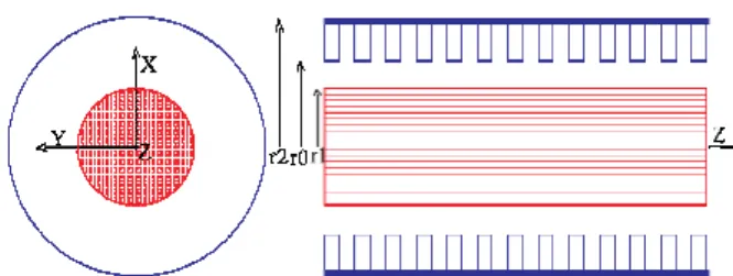
Fig 1 shows the anisotropic-dielectric-loaded corrugated guide. The anisotropic dielectric has optical

Anisotropic-dielectric-loaded corrugated

guide

K.C.C.O.Senhorini, J.R.Descardeci,

Department of Electrical Engineering, Federal University of Tocantins, UFT. Palmas, Brazil, kathy@uft.edu.br,ricardo@uft.edu.br

J.R.Bergmann

axis in the z-direction. r1 is the dielectric rod radius, r0 is the corrugated guide radius (without

corrugations) and r2 is r0 plus corrugation depth.

Fig. 1. Geometry of Anisotropic-dielectric-loaded corrugated guide.

B. Suggested technique to produce uniaxial anisotropy

It is suggested to produce anisotropy in the dielectric rod by perforating the dielectric in the axial

direction (z-direction). The dielectric can be a PTFE (Polytetrafluoroethylene is a synthetic fluoropolymer of tetrafluoroethylene. It is most well known by the DuPont brand name Teflon) type material with a very good homogeneity. The idea is to achieve a more homogeneous and structurally

strong material than the dielectric foam. The values of permittivity in the transversal (x and y-directions) and axial direction are given by the equations [5]:

0 0

0

0

0

0

0

0

t

t r

z

ε

ε

ε

ε

ε ε

ε









=

_

_

=









(1)

where:

(

2 ( 1) / 2

) (

( 1)

)

1 ( 1)

t r r r r

z r

C C

C

ε

ε

ε

ε

ε

ε

ε

 = + − − −

 

= + −

 (2)

and:

r

ε

- is the tensor of the relative dielectric permittivity

t

ε

- is the transversal relative dielectric permittivity

z

ε

- is the tangential relative dielectric permittivity

where

AT – is the transversal area of the dielectric rod

AF - is the transversal area of the holes (it is assumed that the holes have the same transversal area)

and N - is the hole numbers.

C. Theoretical Formulation

Considering the geometry of the problem shown in Figure 1, in region r < r0, the longitudinal field

components Ez and Hz must satisfy the wave equation and the solutions are given by a mode

expansion inside and outside the rod.

Inside the dielectric rod (r<r1):

2

( , , ) ( ) cos( ) z

Zn n n

Ei r

φ

z ₌K A J Kr n e

φ

−γ

(4)

2

( , , ) ( ) sin( ) z

Zn i n n

Hi r

φ

z ₌ y K B J Kr n e

φ

−γ

(5)

with

2 2 2

0 z

K =k

ε

+

γ

(6)

Outside the dielectric rod (r1<r<r0):

(

)

2

1 1 1

( , , )

(

)

(

) cos(

)

z

Zn n n n n

Eo

r

φ

z

₌

k

C J k r

₊

D Y k r

n e

φ

−γ

(7)

(

)

2

1 1 1

( , , )

(

)

(

) sin(

)

z

Zn o n n n n

Ho

r

φ

z

y k

E J k r

F Y k r

n e

φ

−γ

=

+

(8)

with

2 2 2

1 0

k =k +

γ

(9)

and

0/ 0

i z o z

y = ε µ ε =y ε is the intrinsic dielectric admittance, yo is the intrinsic air admittance, γ is

the propagation constant, with γ=α+jβ≅ jβ=γ_Z, for the lossless case.

k

0 is the free space wave

number. J x_n( ) and Y x_n( ) are Bessel functions of first and second kind of order n, respectively.

The φ-component of the fields are given by:

0

( , , ) ( ) ' ( ) sin( ) z

n n i n n

n

Ei r z A J Kr j y KB J Kr n e

r

γ φ

γ

φ



ωµ



φ

−

=_ + _

0

( , , ) i ( ) ' ( ) cos( ) z

n n t n n

n y

Hi r z B J Kr j KA J Kr n e

r

γ φ

γ

φ



ωε ε



φ

−

= −_ + _

  (11)

(

)

(

)

1 1

0 1 1 1

(

)

(

)

( , , )

sin(

)

' (

)

' (

)

n n n n z

o n n n n

n

C J k r

D Y k r

r

Eo r

z

n e

j

y k E J

k r

F Y

k r

γ φ

γ

φ

φ

ωµ

−





+

+





=

_

_



₊







(12)

(

)

(

)

1 1

0 1 1 1

(

)

(

)

( , , )

cos(

)

' (

)

' (

)

o

n n n n z

n n n n

n y

E J k r

F Y k r

r

Ho r

z

n e

j

k C J

k r

D Y

k r

γ φ

γ

φ

φ

ωε

−





+

+





= −

_

_



₊

₊







(13)

Next, the boundary conditions are applied considering the surface-impedance approach instead of the

use of space harmonics. This is a good approximation for slot width smaller than a tenth of a wavelength [2]. The approximation improves as the number of slots per wavelength increases. Application of boundary conditions will produce a system of equations that must be numerically

solved to obtain the propagation constant for the hybrid modes HE and EH. The system of equations is presented bellow:

11 12 13 14 15 16

21 22 23 24 25 26

31 32 33 34 35 36

41 42 43 44 45 46

51 52 53 54 55 56

61 62 63 64 65 66

0 0 0 0 0 0 n n n n n n A B C D E F

α

α

α

α

α

α

α

α

α

α

α

α

α

α

α

α

α

α

α

α

α

α

α

α

α

α

α

α

α

α

α

α

α

α

α

α

                        =                        _{ }     _{ }     (14) where:

11 12 21 22 32 35 36 41 43 44

0

α

=

α

=

α

=

α

=

α

=

α

=

α

=

α

=

α

=

α

=

(15)

13 1 0

0

( )

n

n

J k r r

γ

α

= (16)

14 1 0

0

( )

n

n

Y k r r

γ

α

= (17)

15

j

0 1

k y J

o

' (

n

k r

1 0

)

α

=

ωµ

(18)

16

j

0 1

k y Y

o

' (

n

k r

1 0

)

2

24 j k1 0Y' (n k r1 0) k Y r Y k r1 S( ) (0 n 1 0)

α

=

ω ε

+ (21)

25 1 0

0

( )

o n

n

y J k r r

γ

α

= (22)

26 1 0

0

( )

o n

n

y Y k r r

γ

α

= (23)

2

31 K J Krn( 1)

α

= (24)

2

33 k J k r1 n( 1 1)

α

= − (25)

2

34 k Y k r1 n( 1 1)

α

= − (26)

2

42 y K J Kri n( 1)

α

= (27)

2

45 y k J k ro 1 n( 1 1)

α

= − (28)

2

46 y k Y k ro 1 n( 1 1)

α

= − (29)

51 1

1

( ) n

n

J Kr r

γ

α

= (30)

52

j

0

y KJ

i

' (

n

Kr

1

)

α

=

ωµ

(31)

53 1 1

1

( ) n

n

J k r r

γ

α

= − (32)

54 1 1 52 0 1

1

( ) ' ( )

n i n

n

Y k r j y KJ Kr

r

γ

α

= −

α

=

ωµ

(33)

55

j

0

y k J

o 1

' (

n

k r

1 1

)

α

= −

ωµ

(34)

56

j

0

y k Y

o 1

' (

n

k r

1 1

)

α

= −

ωµ

(35)

61

j

0 t

KJ

' (

n

Kr

1

)

62 1 1

( ) i n

n

y J Kr r

γ

α

= − (37)

63

j

0 1

k J

' (

n

k r

1 1

)

α

=

ωε

(38)

64

j

0 1

k Y

' (

n

k r

1 1

)

α

=

ωε

(39)

65 1 1

1

( ) o n

n

y J k r r

γ

α

= (40)

66 1 1

1

( ) o n

n

y Y k r r

γ

α

= (41)

and Y r_S( )₀ is the surface admittance given by:

0 0 0 2 0 2 0 0

0 0

0 0 0 2 0 2 0 0

' (

) (

)

(

) ' (

)

( )

(

) (

)

(

) (

)

n n n n

S

n n n n

J

k r Y k r

J k r Y

k r

Y r

jy

J k r Y k r

J k r Y k r



−



= −





−





(42)

The far-fields are obtained by applying the Fourier Transform in the aperture tangential fields [6].

0

2

'sin cos( ')

0 0

'

'

'

r jkr rad

E

C

E e

r dr d

π

θ φ φ

θ θ

φ

−

=

∫ ∫

(43)

0

2

'sin cos( ')

0 0

'

'

'

r jkr rad

E

C

E e

r dr d

π

θ φ φ

φ φ

φ

−

=

∫ ∫

(44)

The co-polar and cross polar fields are obtained by using Ludwig’s third definition [7].

III. SIMULATEDRESULTS

Some particular cases were simulated to validate the theoretical development presented in this article

and to analyze the dielectric rod anisotropy effect in the structure. The particular geometry used has r1

= 0.05054m, r0 = 0.06317m and corrugation depth d = 0.014m. Initially it was considered an isotropic

dielectric rod with εr=1.05 in order to compare the results with the existing literature [4]. Fig 2

presents the simulated results. As it was expected, the two curves (corrugated [4] and

dielectric-corrugated) are very close. The dielectric-corrugated-guide curve for the HE11 mode crosses (β/k0)=1

tending to square root of εr, but don’t pass this value for a wide frequency band. In other simulation,

an isotropic dielectric rod with εr = 10.3 (Alumina Ceramic) [8] is perforated with 450 holes

curves, for the two main modes, are presented in the Fig 3. In this figure, it is also presented the dispersion curves for the isotropic dielectric rod with εr = 3.745. The isotropic permittivity value εr =

3.745 can be obtaining with: “Cross linked poly styrene / ceramic powder-filled, Silicone resion

ceramic powder-filled, airwith rexolite standoffs fusedquartz” [8].

0 10 20 30 40 50 60 70 80 90 100 110 120

0,0 0,2 0,4 0,6 0,8 1,0 1,2 1,4 1,6 1,8

β

/k

0

k0

CORR+DIEL_ ISO_1.05 CORRUGADO EH11

HE11

Fig. 2. Simulated dispersion curves for the degenerate case of an isotropic dielectric rod with εr=1.05, and for

the hollow cylindrical corrugated guide [4]. r1=0.05054m, r0=0.06317m and corrugation depth d=0.014m.

0 10 20 30 40 50 60 70 80 90 100 110 120

0,0 0,2 0,4 0,6 0,8 1,0 1,2 1,4 1,6 1,8

CORR+DIEL_ISO_3.745 CORR+DIEL_ANISO_3.745

β

/k

0

k0 HE11 EH11

Fig. 3. Simulated dispersion curves. Parameters: r1=0.05054m, r0=0.06317m and corrugated depth d=0.014m.

Anisotropy was created by inserting 450 axial holes, with diameter φ=4 mm, in the dielectric with εr=10.3

resulting εt=2.737 and εz=3.745. Isotropic dielectric εr=3.745.

The isotropic simulated curves, presented in Fig 3, were compared and agreed with existing literature [2-4]. When dielectric anisotropy is present, the HE11 dispersion curve moves to the right. This result

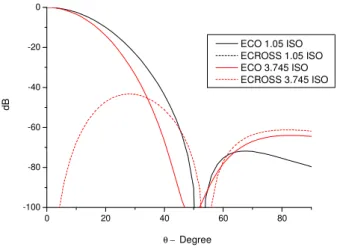
The co- and cross polar radiated far-fields for both cases of Fig 3 (isotropic and anisotropic) are

presented in Fig 4. In this simulation it was considered f=5.252 GHz (

k

₀=110) and only the presence of the main mode HE11.

0 20 40 60 80

-100 -80 -60 -40 -20 0

d

B

θ − Degree

ECO 3.745 ANISO ECROSS 3.745 ANISO ECO 3.745 ISO ECROSS 3.745 ISO

Fig. 4. Co-polar and cross-polar radiated fields for the balanced hybrid HE11-mode. Plane 45°. Parameters:

r1=0.05054m, r0=0.06317m and corrugation depth d=0.014m. Anisotropy created by 450 holes axial, with

diameter φ=4mm, in the dielectric with εr =10.3 resulting εt=2.737 and εz=3.745. Isotropic dielectric εr =3.745.

0 20 40 60 80

-100 -80 -60 -40 -20 0

θ − Degree

d

B

ECO 1.05 ISO ECROSS 1.05 ISO ECO 3.745 ISO ECROSS 3.745 ISO

Fig. 5. Co-polar and cross-polar radiated fields. Plane 45°. Parameters: r1=0.05054m, r0=0.06317m and

corrugated depth d=0.014m. Isotropic dielectric εr=3.745 and isotropic dielectric εr=1.05.

In the Fig 5 are showed the co- and cross polar radiation curves for the isotropic cases of εr = 1.05

and εr = 3.745 for the same frequency utilized in the figure 4. In this figure, it is observed cross

IV. CONCLUSIONS

This paper presented the characteristic equation developed for the corrugated cylindrical guide with

anisotropic dielectric rod. The hybrid modes dispersion curves generated by this characteristic equation were tested with the degenerated case of a hollow cylindrical corrugated guide by using an

isotropic dielectric with: εr = 1.05. The results were presented in the Figure 2 and showed very close

agreement. This was expected, since the dielectric was very close to unity. In this case the structure is almost the same the structure of the corrugated guide. This paper also presented and compared

simulated dispersion curves for the degenerated case of isotropic dielectric with εr = 3.745 and the

case of an anisotropic dielectric with εz = 3.745 and εt = 2.737. This anisotropic material was created

by perforating an isotropic material with εr = 10.3 according to the technique describe in this article.

In both cases the dispersion curves were identical for the mode EH11 and little difference were observed for the mode HE11. The anisotropic HE11 mode presented cut-off value higher than

isotropic one. This is because of the smaller permittivity in the transversal direction. The radiation pattern of Figure 4 shows that the anisotropy effect created an increment of approximately 3dB in the cross polarization level. The co-polar radiated field presented lower level second lobe for the

anisotropic case. This effect is very interesting and demands more study for its understanding. From the curves presented in Figure 5, it can be verified that the cross polarization were significantly worse

with the highest permittivity isotropic dielectric inclusion. It is predictable, because the structure with

εr = 1.05 is an structure similar to the hollow cylindrical corrugated guide with corrugation depth d =

λ/4, for this case excellent levels of cross polarization are expected. This paper also presented a

technique to reduce the relative permittivity and generate uniaxial anisotropy from an homogeneous isotropic dielectric. The objective is to obtain a material more homogeneous and

mechanic-structurally better than the dielectric foam. The anisotropy created by this technique showed little effect in the dispersion curves and radiation patterns simulated examples. More detailed studies are

being carried out to improve the conclusions on the anisotropic effect in the proposed guide.

ACKNOWLEDGMENT

The authors would like to acknowledge the Brazilian agencies: CNPq and CAPES-PROCAD.

REFERENCES

[1] P.D.Potter, “A new horn antenna with suppressed sidelobes and equal beamwidth,” Microwave J., pp. 71–78, June 1963.

[2] P. J. B. Clarricoats and A. D. Olver, Corrugated Horns for Microwave Antennas, London: Peter Peregrinus Ltd, IEE, 1984.

[3] A. D. Olver, P. J. B. Clarricoats and L. Shafai, Microwave Horns and Feeds, London: IEEE Press, Inc., New York, 1994.

[4] P.J.Clarricoats, J.R.Descardeci and A.D.Olver, “A Low Crosspolar Feed for Broadband Application,” 1988- URSI-International Symp. On Electromagnetic Theory, Thessaloniki USRI, 1988, v.1. pp. 110-119.

[5] A.V.Ghiner and G.I.Surdutovich, “Method of Integral Equations and an Extinction Theorem for Two-Dimensional Problems in Nonlinear Optics,” Physical Review A,vol 50, N.1, July 1994, pp.714-723.

[6] C.A.Balanis, Advantage Engineering Electromagnetic, USA, John Wiley & Sons, 1989.