Simulating a Chaotic Process
Ricardo L. Viana, Jos´e R. R. Barbosa
∗,
Departamento de F´ısica, Universidade Federal do Paran´a81531-990, Curitiba, Paran´a, Brazil
Celso Grebogi,
Instituto de F´ısica, Universidade de S˜ao Paulo 05315-970, S˜ao Paulo, S˜ao Paulo, Brazil
and Antˆonio M. Batista,
Departamento de Matem´atica e Estat´ıstica, Universidade Estadual de Ponta Grossa, 84033-240, Ponta Grossa, Paran´a, Brazil
Received on 7 April, 2004
Computer simulations of partial differential equations of mathematical physics typically lead to some kind of high-dimensional dynamical system. When there is chaotic behavior we are faced with fundamental dynamical difficulties. We choose as a paradigm of such high-dimensional system a kicked double rotor. This system is investigated for parameter values at which it is strongly non-hyperbolic through a mechanism called unstable dimension variability, through which there are periodic orbits embedded in a chaotic attractor with different numbers of unstable directions. Our numerical investigation is primarily based on the analysis of the finite-time Lyapunov exponents, which gives us useful hints about the onset and evolution of unstable dimension variability for the double rotor map, as a system parameter (the forcing amplitude) is varied.
1
Introduction
Computer simulations of partial differential equations are a main tool in the hands of physicists, playing an increasingly important role in their formation [1]. There are plenty of physical problems where computer simulations have an out-standing position, like in the study of turbulence in fluids and plasmas [2], percolation [3], statistical mechanics [4], and molecular dynamics [5], just to cite a few. Many nu-merical methods for nunu-merical solution of partial differen-tial equations rely on some form of discretization of space and/or time, such that those methods boil down to a system of coupled ordinary differential equations or coupled maps, in the case of a continuous or discrete time variable, respec-tively [6].
Nonlinear dynamical systems, including many par-tial differenpar-tial equations of physical interest, commonly present chaotic motion, i.e. extreme sensitivity to initial conditions [7]. Since there are unavoidable errors inherent to the process of discretizing a partial differential equation, besides the usual one-step integration errors, the computer simulation of such equations may lead to fundamental dy-namical difficulties. One of the aims of the present paper is to present the basic ideas and results underlying the study of the dynamical problems related to high-dimensional
sys-tems undergoing chaotic motion.
We will choose as a paradigm of a high-dimensional dy-namical system a mechanical system consisting of a double rotor subjected to periodic impulsive excitation, in which we adress the most severe of those dynamical difficulties, the so-called unstable dimension variability [8]. The ap-proach we choose to investigate the onset, evolution and ef-fects of unstable dimension variability in dynamical system is to consider the behavior of their numerically computed finite-time Lyapunov exponents.
Finite-time, or time-n, Lyapunov exponents are obtained exactly in the same way as the usual exponents, but over a finite time interval instead of the infinite-time limit al-ways supposed in calculations [9]. Obviously, in practice any computed exponent is a finite-time one, but here we are concentrating in very small time intervals, in then = 1to 100 range. The usefulness of finite-time exponents result from their interpretation as local expansion or contraction rates of a given trajectory during a small interval of time [10, 11]. Hence, it is particularly sensitive to dynamical situations wherein the phase space presents a complicated structure of invariant sets with different numbers of stable and unstable directions.
This is the case, for example, of strongly non-hyperbolic dynamical systems presenting unstable dimension
ity, which is characterized by the simultaneous occurrence, within the same invariant chaotic set, of unstable periodic orbits with a different number of unstable eigendirections [12]. It turns out that, as a typical chaotic trajectory wan-ders through the invariant set, it experiences alternate con-tractions and expansions with respect to the eigendirection which varies from point to point in the set. This is reflected in a fluctuating behaviour (around zero) of the correspond-ing finite-time Lyapunov exponent, since it is the local ex-pansion rate for that eigendirection.
We remark that there are severe consequences of un-stable dimension variability on the validity of numerically generated trajectories (which have small yet unavoidable one-step errors), since they fail to be shadowed by fiducial chaotic trajectories for a sufficiently large timespan [13]. In cases where a physical system is found to present unstable dimension variability we are thus able to closely follow a computer-generated trajectory for a time so short that it can-not be taken individually as a faithful representation of the actual dynamical behavior we are investigating [14]. Even statistical averages computed with help of non-shadowable chaotic trajectories may be doubtful since tiny errors may be largely amplified by system dynamics [15].
Unstable dimension variability was first described in a dynamical system of physical interest, a periodically kicked double rotor [16], and later on it was recognized that a fin-gerprint of unstable dimension variability, when it occurs at all, is the fluctuating behavior (around zero) of the finite-time Lyapunov exponent closest to zero [17]. It must be stressed, however, that it may happen that such exponents may fluctuate in such way without being a clearcut charac-terization of unstable dimension variability, since this fluc-tuations can come from other sources of non-hyperbolic be-havior [18]. Hence, the onset and evolution of unstable di-mension variability should be also sought for in the stability analysis of unstable periodic orbits embedded in the invari-ant chaotic set, and which support the ergodic measure of the orbits whose initial conditions lie in that set.
Nevertheless, the analysis of finite-time Lyapunov expo-nents has been proved to be very useful to give numerical insights on the onset and evolution of unstable dimension variability, especially in high-dimensional dynamical sys-tems (like coupled oscillator and map lattices), where un-stable dimension variability has been found to be very com-mon [19]. The purpose of this paper is to investigate the onset and evolution of unstable dimension variability in the kicked double rotor map, as one system parameter (the forc-ing amplitude) is varied. We will base our analysis on the be-havior of the finite-time Lyapunov exponents, as well as on the stability analysis, whenever it is possible due to the high-dimensionality of the system, of the relevant low-period un-stable orbits. Two basic issues are highlighted through this work: the onset of unstable dimension variability, which we conjecture to coincide with the onset of chaotic behavior it-self; and the point where unstable dimension variability is most intense, namely, when occurs a codimension-one bi-furcation within the chaotic set.
The rest of this paper is organized as follows: Section II presents the kicked double rotor system and the
correspond-ing map equations, as well as some aspects of its chaotic dynamics. Section III discusses the onset and evolution of unstable dimension variability, when a system parameter is varied. The last section contains our conclusions.
2
Kicked double rotor map
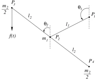
The kicked double rotor system consists of two rods of neg-ligible mass and of lengthsℓ1andℓ2, respectively (Fig. 1).
The former rod, which has a point massm1attached to one
of its ends, is pivoted at the point P1, and its angular
po-sitionθ1 ∈ [0,2π)is measured with respect to a reference
line. The latter rod, with length2ℓ2, is pivoted at its
mid-pointP2and has two point massesm2/2attached to its free
ends. The corresponding angular position,θ2, is measured
with respect to a line parallel to the first reference line. We do not consider any gravity effects on this system (for ex-ample, it can move on a horizontal plane without friction).
An impulsive force
f(t) =f0
∞ X
k=1
δ(t−kT), (1)
with amplitude f0 ≥ 0and periodT, is applied at one of
the free ends, in a direction parallel to the reference line (cf. Fig. 1). Dissipation in this system occurs at the pivoting pointsP1andP2by means of viscous frictional forces. The
friction atP1, with damping coefficientν1>0, slows down
the first rod at a rate proportional to its angular velocityθ˙1.
The friction at the other pivot,P2, slows down the second
rod (but accelerates the first one) according to the relative angular velocitiesθ˙2−θ˙1, with damping coefficientν2>0.
2
m
22
m
2P
1l
P
f(t)
4
P
3l
2m
1l
12 2
θ
1
θ
P
2Figure 1. Sketch of a kicked double rotor.
We introduce the following discretized dynamical vari-ables:
Xn = µ
(x1)n
(x2)n
¶ = lim
ε→0 µ
θ1(nT+ε)
θ2(nT+ε)
¶ (2)
(n = 0,1,2,· · ·),T being the period of the delta-function excitation; and
Yn = µ
(y1)n
(y2)n
¶ = lim
ε→0 µ ˙
θ1(nT+ε) ˙
θ2(nT+ε)
¶ (3)
being the corresponding discretized angular velocities. Given the angular positions and velocities at timen, one can obtain the corresponding variables at the next instant
n+ 1by using the following map (further details on the ob-tention of this map can be found in Ref. [16]):
Xn+1 = MYn+Xn (4)
Yn+1 = LYn+G(Xn+1) (5)
where the nonlinear functions are
G(X) = µ
(f0ℓ1/I) sinx1 (f0ℓ2/I) sinx2
, (6)
andI = (m1+m2)ℓ21=m2ℓ22is the moment of inertia of
the rotor.
The2×2constant matricesLandMare such that
L=I2+AνM, (7)
whereI2is the identity matrix, and
Aν= µ
−(ν1+ν2) ν2
ν2 −ν2
¶ , (8) with M= 2 X j=1
Wjexp (sjT)−1
sj
, (9)
where
s1,2=− 1
2(ν1+ 2ν2±∆), (10)
are the eigenvalues ofAν, with∆ ≡pν12+ 4ν22, and we have defined the following matrices
W1= µ
a b b d
, W2= µ
d −b
−b a
, (11)
with constant entries
a≡ 12³1 + ν1 ∆ ´
, d≡12³1−ν∆1´, b≡ −ν∆2. (12)
In the following, we simplify matters, without loss of generality, by taking convenient numerical values for the physical magnitudes involved:
ℓ1= 1/
√
2, ν1=ν2=T =I=m1=m2=ℓ2= 1,
such that
L= µ
0.2414 0.2726 0.2726 0.514
, M= µ
0.4860 0.2133 0.2133 0.6993
.
(13) As already mentioned, the control parameter to be varied is the driving amplitudef0.
The dynamics of the kicked double rotor map (KDRM) is structured on their fixed points and periodic orbits. Due to theyi → −yi symmetry of the kicked double rotor map
it turns out that the planey1 =y2 = 0is an invariant
sub-space of the system, embedded in its four-dimensional phase space. Any initial conditions belonging to this plane will generate orbits which cannot escape from it as time evolves. Hence, at least some of the fixed points of the map, given by
X∗
= MY∗
+X∗
(mod2π) (14)
Y∗
= LY∗
+G(X∗
) (15)
must lie on this invariant subspace. The solutions of the above equations can be classified in one-parameter families [16]
X∗
= Ã
x(n1,n2,q)
1∗
x(n1,n2,q)
2∗
!
Y∗
= Ã
y(n1,n2)
1∗
y(n1,n2)
2∗ !
(16)
where (n1, n2) are integer rotation numbers, and q = 1,2,3,4. In fact, four of these fixed points (X∗
,Y∗
) lie on they1 = y2 = 0 plane. We will analyze particularly
the fixed point with n1 = n2 = 0 and p = 4, called
P= (x∗
1 =π, x
∗
2=π, y
∗
1 = 0, y
∗
2 = 0).
A representative part of the bifurcation diagram for the kicked double rotor map is depicted in Fig. 2, where one of the dynamical variables, namely the angular position of the second rod,x2, is plottedversusthe kick strengthf0in
the interval[4.0,7.0]. For small values off0we observe the
stable fixed point,P, which undergoes a period doubling bifurcation atf0 ≈4.27producing a stable period-2orbit.
The latter is followed, for higher forcing amplitudes, by a period-doubling cascade leading to chaos for f0 ≈ 6.75.
The chaotic bands merge together and eventually fuse them-selves into a single large chaotic band, atf0 ≈ 6.85due
to a crisis triggered by the collision of the two-band chaotic attractor with some unstable orbit.
4 5 6 7
f 0 0 1 2 3 4 5 6 x2
Figure 2. Bifurcation diagram ofx2 versusthe control parameter
f0∈[4.0,7.0].
a saddle-node bifurcation (i.e., there is also a companion
unstable periodic orbit). This orbit undergoes a period-doubling cascade (not shown in the figure due to insufficient graphical resolution) leading to a chaotic motion suddenly interrupted atf0 ≈ 5.4 due to a crisis (caused by the
col-lision between the chaotic attractor and the unstable orbit created at the saddle-node bifurcation). Another coexisting periodic orbit appears and disappears in the narrow interval [6.2,6.3].
3
Unstable dimension variability in
the kicked double rotor map
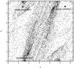
To introduce the key question to be discussed in this pa-per, let us make a simple numerical experiment with the kicked double rotor map: we choose a given value of the control parameter and an initial condition for which the map is known to generate a chaotic orbit. Next we iterate the map for a given number of times, using both single and double precision (see Fig. 3). It is seen that, after no more than18map iterates, the resulting orbits are far apart by a distance comparable to the length scale used of that phase space region. Since the only difference between these tra-jectories (∼ 10−8
) has been the truncation furnished by the computer arithmetics we have chosen, one could under-standably regardbothorbits as equally suspicious, because a third and different trajectory would result from using an-other (e.g., quadruple) numerical precision. As this problem is not likely to end with an ever increased arithmetical pre-cision, one could ask whether or not should we trust those computer-generated orbits?
0 1 2 3 4 5 6
x1 0
1 2 3 4 5 6
x2
single precision initial condition
double precision
Figure 3. Projection, on the(x1, x2)plane, of the phase points of two chaotic trajectories arising from the same indicated initial con-dition(5.5,5.7,0.0,0.0)and iterated 18times using single and double precision, for the KDRM(f0= 7.5).
This is obviously nothing but a consequence of the chaotic nature of the orbits. Consider that, for the value
of control parameter used in plotting Fig. 3, the maximal Lyapunov exponent of the KDRM isλ1 ≈ 1.1[16]. The
phase-space distance between the single and double preci-sion trajectories after one iterate, which is of the order10−8
, grows exponentially as the timenincreases at a rate equal to the maximal Lyapunov exponent; in that way, the number of iterations for which the distance increases to a number of order1is
1 λ1
ln µ
1
10−8
¶ ∼17,
in accordance with the result illustrated by Fig. 3.
In spite of this, it is far from trivial to get the answer to the question about whether or not those computer-generated chaotic orbits are meaningful. In fact, the efforts to come to a comprehensive understanding of such problems have stimulated a branch of pure mathematics called “shadowing theory” [13]. There has been proved that only hyperbolic systems are shadowed by an arbitrarily large (in fact, infi-nite) timespan [20, 21]. When the dynamics fail to be hy-perbolic due to glitches caused by near-tangencies between stable and unstable manifolds of an unstable orbit, it can still be argued that shadowing is possible during a timespan of the orderδ−1/2
, whereδis the magnitude of the one-step errors commited during numerical computation of that orbit [22]. If the system is non-hyperbolic due to unstable dimen-sion variability, however, the shadowing time depends on the statistical properties of the finite-time Lyapunov exponents, and may be so short that no useful prediction can come from single chaotic trajectories [15].
In order to investigate the onset and evolution of unsta-ble dimension variability in the kicked douunsta-ble rotor map, we will focus on the first representative chaotic attractor of the double rotor, which appears atf0 ≈ 6.75[see Fig. 2],
where the maximal Lyapunov exponentλ1crosses zero and
becomes positive [16]. Exception being made to periodic windows, such as those occurring at7.0 <∼ f0 <∼ 7.2and
around8.2, the exponentλ1is almost always positive
indi-cating a reasonably steady chaotic dynamics for the system. As the forcing amplitude is further increased, it turns out that the second Lyapunov exponent,λ2, builds up monotonically
and crosses zero atf∗
0 = 8.1104126. This is recognized as
the onset of hyper-chaos in the system, since there is more than one positive exponent. The unstable fixed pointP is embedded in this chaotic attractor.
Computing the eigenvalueξ2(the closest to unity in
ab-solute value), of the linearized map for the fixed pointP, there results that, whenf0<∼f0∗= 8.1104126,Ppossesses
three stable and one unstable direction, henceds(P) = 3
anddu(P) = 1. Evaluating the eigenvalueξ2in the
neigh-borhood of the hyper-chaotic transition point f∗
0 (Fig. 4),
there occurs a period-doubling bifurcation. For f0 >∼ f0∗
the fixed pointP acquires two stable and two unstable di-rections, i.e., its unstable dimension becomesdu(P) = 2.
does not contain all points belonging to the attractor. In ad-dition to this set of periodic orbits withdu = 2, there
re-mains an infinite number of other periodic orbits that con-tinue to have unstable dimensiondu = 1. Since these sets
are densely intertwined in the attractor, a typical chaotic tra-jectory will approach points with one or two unstable direc-tions.
7.98 8 8.02 8.04 8.06 8.08 8.1 8.12
f0 -1.01
-1 -0.99 -0.98 -0.97 -0.96
s2
Figure 4. Eigenvalue of the Jacobian matrix of the KDRM as a function of the control parameterf0near the emergence of
hyper-chaos.
This is a direct evidence that unstable dimension vari-ability occurs for the chaotic attractor of the double rotor whenf0>∼f0∗. However, as we will see in the next section,
the onset of unstable dimension variability occursbeforef∗
0.
This is because there may occur variations on the unstable dimension of other fixed points or periodic orbits embedded in the chaotic attractor, before this happens for this selected fixed pointP. The problems with shadowability of numer-ical trajectories, in this case, follow from this complicated mixture of high-dimensional saddles and repellers. Con-sider a hyper-sphere in the four-dimensional phase space filled with initial conditions, whose evolution according to the double rotor map, generates “true”, or fiducial chaotic trajectories. When this sphere approaches a given saddle (du = 1), it will shrink along three stable directions and
elongate along one unstable direction, becoming a cigar-like tube centered at the saddle (Fig. 5) [23].
A numerically generated, or pseudo-trajectoryA, will be contained inside this cigar-like tube of radiusδ(δbeing the one-step error level commited during numerical iteration of the map), and this tube will also contain a true orbitBwhich will shadowA, since their pointwise distance is bounded by
δ. After a further number of iterations, the cigar-like tube will approach a repeller(du = 2)and will rapidly expand
along the extra unstable direction. In this case, the pointwise
distance betweenAandBwill be no longer bounded and in-creases exponentially along the new unstable dimension. As a consequence,Awill be no longer shadowed byB, for they diverge exponentially with time. Since the sets of saddles and repellers are dense in the chaotic attractor, the time dur-ing which we preserve shadowdur-ing may be extremely short.
repeller (d = 2)
δ
A B
A B
saddle (d = 1) u
u
Figure 5. Schematic illustration of the evolution of a cigar-like tube of trajectories (which cross-section in the page plane is a circle) in presence of unstable dimension variability. The direction perpen-dicular to the page is repulsive.
These observations about expansion and contraction of phase space volumes can be made more quantitative by introducing the corresponding finite time Lyapunov expo-nents. Letf(x)be ad-dimensional map, wherenis a pos-itive integer, such thatDfn(x0)is the Jacobian matrix of then-times iterated map, with entries evaluated at the initial conditionx0. Suppose that the singular values ofDfn(x0) are ordered:ξ1(x0, n)≥ξ2(x0, n). . .≥ ξn(x0, n). Then,
thek-th time-nLyapunov exponent for the pointx0is de-fined as [24]
λk(x0, n) = 1
nln||Df
n(x
0).vk||, (17)
wherevkis the eigenvector corresponding toξk(x0, n). The infinite time-limit of the above expression is the usual Lyapunov exponent
λk(∞) = lim n→∞λk(
x0, n) (18)
Although the time-nexponentλk(x0, n)generally takes on
a different value, depending on the point we choose, the in-finite time limit takes on the same value for almost allx0 with respect to the natural ergodic measure of the invariant set. For the kicked double rotor map there are four time-n
exponents, ordered asλ1(n) > λ2(n) > λ3(n) > λ4(n),
but we will be interested only in the closest to zero, which in this case turns out to beλ2(n).
A numerical indication of unstable dimension variabil-ity is the fluctuating behavior (around zero) of the time-n
average) and others for which it is transversely repelling (also on average). This is properly quantified by the time-n
Lyapunov exponent closest to zeroλ2(n): when the
trajec-tory sections of durationnare such that there is an average contraction (expansion) along its eigendirection, the corre-sponding time-nexponent is negative (positive). Hence, if the chaotic invariant set displays unstable dimension vari-ability, there will be length-nsections of a typical trajectory for whichλ2(n)is positive, even when the infinite-time
ex-ponentλ2(∞)is negative. This suggests the use of a
prob-ability distributionP(λ2(n)), such thatP(λ2(n))dλ2(n)is
the probability that the second time-nexponent lies between
λ2(n)andλ2(n) +dλ2(n).
-1 0 1
λ2(10)
0 0.5 1 1.5 2 2.5
P(
λ2
)
f0=8.4 f0=8.0
f0=7.6 f0=7.0
f0=6.9
f0=9.0
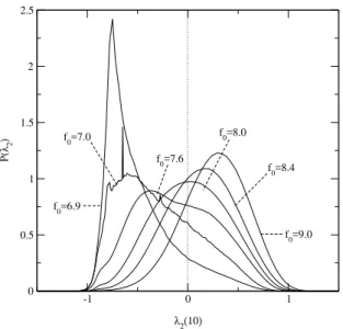
Figure 6. Probability distribution for the second finite-time Lya-punov exponent,λ2(10), for the kicked double rotor map.
We can obtain a numerical approximation for this prob-ability distribution, for the double rotor map, by means of a histogram drawn on a large number of trajectories of length
nfrom randomly chosen initial conditions. In Fig. 6, we show a few distributions of time-10exponents, obtained for different values of the forcing amplitudef0, chosen in a
pa-rameter interval roughly centered at the onset of hyper-chaos (f∗
0), the bell-shape ofP(λ2(n))being more evident as we
approach this point. The maxima of the distributions drift towards positive values, asf0 varies in the vicinity of the
hyper-chaos transitionf∗
0. Fig. 7 plots the average values
of the distributions of the time-10exponents along the four eigendirections, < λi(n) >,i = 1,2,3,4. This figure is
very similar to the corresponding diagram for the infinite-time Lyapunov exponents [16, 23]. In fact, for Gaussian distributions it follows that [8]
hλ2(x0, n)i=
R+∞
−∞ λ2(x0, n)P(λ2(x0, n))dλ2 R+∞
−∞ P(λ2(x0, n))dλ2
=λ2(∞)
(19)
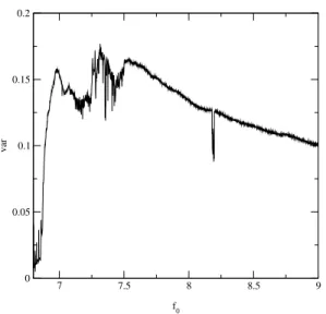
Figure 7 points out that the average time-n exponent crosses zero at a constant rate in the neighborhood of the hyper-chaos transition. Since the distributions depicted in Fig. 6 have most of theλ2(n)-values in the[−1,+1]range,
there results a considerable distortion of these distributions, with respect to a Gaussian shape. This is confirmed by Fig. 8, which plots the variance σ2
n of the P(λ2(n))
dis-tributions in the same range, showing a highly fluctuating behavior before hyper-chaos, and a mostly smooth decrease before it. In other dynamical systems for which unstable dimension variability has been studied [25, 26], the distrib-utions of the corresponding time-nexponent of interest, be-sides being Gaussian-shaped, drift towards positive values without noticeable distortion of shape.
7 7.5 8 8.5 9
f0 -3
-2 -1 0 1 2
averages
<λ1(10)>
<λ2(10)>
<λ3(10)>
<λ4(10)>
Figure 7. Average time-10Lyapunov exponents for the kicked dou-ble rotor map, as a function of the forcing amplitude.
A quantity of interest is the fraction of positive values of
λ2(n)
φ(n) = R∞
0 P(λ2(n))dλ2(n)
R+∞
−∞ P(λ2(x0, n))dλ2
. (20)
We can obtain an approximate location for the onset of un-stable dimension variability, as a system parameter is con-tinuously varied, as the parameter value for which the frac-tionφ(n)becomes nonzero. Fig. 9 depicts a numerical ap-proximation of this fraction for the double rotor map, in-dicating is apparently at a valuef0 = (f0)C ≈ 6.8. The
7 7.5 8 8.5 9
f0 0
0.05 0.1 0.15 0.2
var
Figure 8. Variance of the second time-10Lyapunov exponents for the kicked double rotor map, as a function of the forcing ampli-tude.
7 8 9
f0 0
0.2 0.4 0.6 0.8
φ
Figure 9. Fraction of positive second time-10Lyapunov exponents for the kicked double rotor map, as a function of the forcing ampli-tude.
The transition to hyper-chaos is identified in Fig. 9 with a positive fraction of50%of the exponents. In fact, Fig. 6 shows, for this value, a distribution with symmetric tails whose maximum crosses theλ2(n) = 0line. When half of
the time-nexponents are negative, given a certain value of
λ2(n)in modulus, say0.2, there is an approximately equal
probability of this value be positive or negative. In other words, the relative weight of local expansions or contrac-tions is roughly the same, what is the worst situation when
one tries to obtain a “true” chaotic trajectory which shadows a numerical one. This argument can be made more precise by assigning these relative contributions of contractions and expansions the weights of unstable periodic orbits with dif-ferent unstable dimensions by computing the natural mea-sure of the chaotic attractor [23, 8].
Hence, the onset of hyper-chaosdoes notcoincide, in general, with the onset of UDV, but the former is rather the point at which the effect of UDV is of maximum strength. This point marks also theblowout bifurcation, at which the chaotic set as a whole loses transversal stability (the eigendi-rection related to λ2, in the double rotor map) [27]. The
parameter interval between the onset of unstable dimension variability and its maximum value ((f0)C < f0 < f0∗ for
the KDRM) is related to thebubbling phenomenon, when the chaotic set is contained in an invariant subspace of the system [28]. Forf0> f0∗, according to Fig. 9, the fraction of
positive exponents continues to increase, and so the contrast between negative and positive values. In this case, the ef-fect of unstable dimension variability (for example, in terms of the shadowability properties of chaotic trajectories) be-comes progressively less pronounced, even though the two higher infinite-time Lyapunov exponents increase in this re-gion. Curiously, it appears that strongly hyper-chaotic tra-jectories are best shadowed than those at the verge of the hyper-chaos transition.
The above observations can be made more quantitative by using the concept ofshadowing time, defined as the time intervalτ during which aδ-pseudo-trajectory is shadowed by a “true” one. Sauer and co-workers [14] have developed a theoretical model of the pseudo-trajectory behavior in the KDRM by considering a biased stochastic diffusion process with a reflecting barrier, the latter playing the role of the one-step errors of level δ which bound the noisy pseudo-trajectory. They estimated an average shadowing time scal-ing as power law,< τ >∼δ−h
, where it has been defined the hyperbolicity exponent [15]
h≡ 2< λσ22(n)> 1
(21)
in terms of the average and variance, respectively, of the dis-tributionP(λ2(1))of the time-1Lyapunov exponent closest
to zero. The latter is related to the variance of the time-n
exponent byσ2 n=nσ21.
In the vicinity of the blowout bifurcation point, where
< λ2(n) >≈ 0, the hyperbolicity exponent is nearly zero,
7 7.5 8 8.5 9 9.5 0
50 100 150
log
10
<
τ>
7.5 7.6 7.7 7.8 7.9 8 8.1 8.2 8.3 8.4 8.5
f0 0
0.25 0.5 0.75 1 1.251.5 1.75 2 2.25 2.5 2.75 3
log
10
<
τ>
Figure 10. Average shadowing time for the kicked double rotor map, as a function of the forcing amplitude. Bottom panel: magni-fication of the interval for which unstable dimension variability is most intense.
4
Conclusions
We have discussed in the last Section the issue of finding “true” trajectories of a chaotic system which can shadow, for a time long enough, a numerically generated pseudo-trajectory of the same model. However, we can also think of these two trajectories as coming fromdifferent models of a same physical phenomenon. If the computer generated tra-jectory is aδ-pseudo trajectory, it can also be regarded as a “true” trajectory which stems from a slightly perturbed ver-sion of the original model. This perturbation, ormodeling error, whose intensity is bounded by a number of the order ofδ, can come from different sources [29].
One possibility is that the trajectory to be shadowed comes from a perturbed version of the model, resulting from either: (i) a parameter imperfect determination; (ii) a small change in the external influence on the model. In the KDRM case, a perturbed version of the model can be due to (i) a small change in the one of the masses or lengths; whereas (ii) could stand for an experimental uncertainty related with the determination of the forcing amplitude, for example. The noisy trajectory is then due to a value off0determined
within an accuracy proportional to δ. Another possibility (iii) is to regard the noisy trajectory as coming from a replica of the KDRM which has been corrupted by an external noise term bounded byδ(this excludes unbounded, e.g. Gaussian, noise).
In both cases, the same concepts of shadowability ap-plied to pairs of trajectories can be extended to pairs of mod-els. One mathematical modelAof a physical phenomenon (like the KDRM) is then said to shadow the mathematical
modelB, which turns to be a slightly perturbed version of A, if the set of all possible outcomes (or trajectories coming from typical initial conditions) from modelAagrees closely with the set of all possible outcomes from modelA. In terms of theǫ-shadowing property of trajectories, this means that foreverytrajectory of modelAthere existsat least one tra-jectory of modelBthatǫ-shadows the particular trajectory of modelA, andvice-versa.
As a consequence, UDV represents a serious obstacle also for model shadowability, since there are trajectories from one model, asA, that do notǫ-shadowanytrajectory from the other one(B)for all but extremely short periods of time. Considering that trajectories from both models do not agree with each other in terms of shadowability, it is un-likely that eitherA orB is a good model for the physical phenomenon it intends to describe, like the kicked double rotor, for no model trajectory shadowsanytrue trajectory of the actual physical system being investigated.
We stress that this uselessness of mathematical models is not due to the inadequacy of the physical hypotheses used in formulating the model, nor the incorrect application (for ex-ample, out of the proper range) of the physical laws, not even due to neglecting subtle but nevertheless key factors under-lying a good modeling. Unstable dimension variability is a mathematical pathology that hampers model shadowability, and which is rather unavoidable, as long as the mechanical system produces chaotic trajectories.
Hence, even though such a model was intended to de-scribe a deterministic system, it will produce at best the same kind of statistical information a stochastic system would yield, as averages and fluctuations. We can call mathematical models of chaotic systems displaying unsta-ble dimension variability aspseudo-deterministic systems, of which the kicked double rotor is a representative exam-ple. Such systems may not display model shadowability in a satisfactory degree for sets of parameter values, and should be avoided when we are making predictions about the future state of the system based on individual trajectories. In these cases, one could resort to time-series analysis methods to reconstruct the attractor from experimental data, like phase space embedding using delay coordinates.
Acknowledgments
This work was made possible through partial financial support from the following Brazilian research agencies: FAPESP and CNPq. C. G. also acknowledges support from Humboldt Foundation. The authors are indebted to S. R. Lopes, S. E. de S. Pinto and J. Kurths for useful discussions and suggestions.
References
[1] S. Koonin and D. Meredith, Computational Physics, Perseus Books, 2002.
[3] D. Stauffer and A. Aharony, Introduction to Percolation The-ory, Taylor and Francis, London, 1994.
[4] S. Moss de Oliveira, P.M.C. de Oliveira and D. Stauffer, Evolution, Money, War and Computers, Teubner, Leipzig-Stuttgart, 1999.
[5] D. C. Rapaport, The Art of Molecular Dynamics Simulation, Cambridge University Press, Cambridge, 2001.
[6] W. H. Press, B. P. Flanger, S. A. Teulkosky, and W. T. Vet-terling, Numerical Recipes: The art of scientific computing. Cambridge University Press, Cambridge, 1986.
[7] L. Lam, Nonlinear Physics for Beginners, World Scientific, Singapore, 1998.
[8] R. L. Viana, C. Grebogi, S. E. S. Pinto, and J. R. R. Barbosa, Int. J. Bifurcat. Chaos13, 3235-3253 (2003).
[9] A. Wolf, J. B. Swift, H. L. Swinney, and J. A. Vastano, Phys-ica16D, 285-317 (1985).
[10] H. Fujisaka, Prog. Theor. Phys.70, 1264 (1983).
[11] A. Prasad and R. Ramaswany, Phys. Rev.E 60, 2761 (1999).
[12] R. Abraham and S. Smale, Proc. Symp. Pure Math. (AMS)
14, 5 (1970).
[13] C. Grebogi, L. Poon, T. Sauer, J. A. Yorke, and D. Auerbach, inHandbook of Dynamical Systems, Ed. B. Fiedler (Elsevier, Amsterdam, 2002) Vol. 2, Chapt. 7.
[14] T. Sauer, C. Grebogi, and J. A. Yorke, Phys. Rev. Lett.79, 59 (1997).
[15] T. Sauer, Phys. Rev. E65, 036220 (2002).
[16] F. J. Romeiras, C. Grebogi, E. Ott, and W. P. Dayawansa, Physica D58, 165 (1992).
[17] S. P. Dawson, C. Grebogi, T. Sauer, and J. A. Yorke, Phys. Rev. Lett.73, 1927 (1994).
[18] H. D. I. Abarbanel, R. Brown, and M. B. Kennel, J. Nonlinear Sci.1, 175 (1991).
[19] Y.-C. Lai, D. Lerner, K. Williams, and C. Grebogi, Phys. Rev. E60, 5445 (1999).
[20] D. V. Anosov, Proc. Steklov Inst. Math.90,1 (1967).
[21] R. Bowen, J. Diff. Eqs.18, 333 (1975).
[22] C. Grebogi, S. Hammel, and J. A. Yorke, J. Complexity3, 136 (1987); Bull. Am. Math. Soc.19, 465 (1988). C. Gre-bogi, S. Hammel, J. A. Yorke, and T. Sauer, Phys. Rev. Lett.
65, 1527 (1990). T. Sauer and J. A. Yorke, Nonlinearity4, 961 (1991).
[23] Y.-C. Lai and C. Grebogi, Int. J. Bifurcat. Chaos 10, 683 (2000); Y.-C. Lai, C. Grebogi, and J. Kurths, Phys. Rev. E
59, 2907 (1999).
[24] E. J. Kostelich, I. Kan, C. Grebogi, E. Ott, and J. A. Yorke, Physica D109, 81 (1997).
[25] R. L. Viana and C. Grebogi, Phys. Rev. E62, 462 (2000).
[26] R. L. Viana and C. Grebogi, Int. J. of Bifurcat. Chaos11, 2689 (2001).
[27] P. Ashwin, J. Buescu, and I. Stewart, Phys. Lett. A193, 126 (1994).
[28] S. E. S. Pinto, R. L. Viana, and C. Grebogi, Phys. Rev. E66, 046213 (2002).
![Figure 2. Bifurcation diagram of x 2 versus the control parameter f 0 ∈ [4.0, 7.0].](https://thumb-eu.123doks.com/thumbv2/123dok_br/18981588.457225/3.892.84.445.475.898/figure-bifurcation-diagram-x-versus-control-parameter-f.webp)