A ZONE-BASED ITERATIVE BUILDING DISPLACEMENT
METHOD THROUGH THE COLLECTIVE USE OF
VORONOI TESSELLATION, SPATIAL ANALYSIS AND
MULTICRITERIA DECISION MAKING
Método iterativo baseado em zonas para deslocamento de edificações utilizando Voronoi Tesselation, análise espacial e tomada de decisão multicriterio.
MELIH BASARANER
Yildiz Technical University Faculty of Civil Engineering Department of Geomatic Engineering
Division of Cartography
Davutpasa Campus TR-34220 Esenler-Istanbul – Turkey E-mail: [email protected]
ABSTRACT
Keywords: Building Displacement; Contextual Generalisation; Voronoi Tessellation; Spatial Analysis; Multicriteria Decision Making.
RESUMO
Neste artigo propõe-se um metodo de deslocamento iterativo baseado na generalização de zonas, como parte da generalização contextual de edificações em mapas topograficos de média escala. O deslocamento é uma operação complicada considerando que deve ser encontrada uma relação entre vários critérios conflitantes. A necessidade para o deslocamento origina-se da incapacidade de manter as distâncias mínimas entre os objetos impostas pelos limites gráficos após o aumento dos objetos do mapa para a escala final. Também é importante manter a acurácia posicional para a esacala e propagar as mudanças aos vizinhos dos objetos preservando ao máximo sua configuração espacial. No método proposto, primieramente é decidido onde e quando iniciar o deslocamento dos edificios com base na análise espacial nas zonas generalizadas criadas pelos agrupamentos de edificações nas quadras. Em seguida, um critério relevante consiste em controlar o deslocamento. Finalmente, os candidatos ao delocamento e os vetores são analisados utilizando Voronoi Tesselation, análise espacial e múltiplos critérios combinados em cada iteração. A avaliação demonstrou que este método é efetivo para deslocamento de edificações baseado em zonas.
Palavras-chave: Deslocamento de Edificações; Generalização Contextual; Voronoi Tessellation; Análise Espacial; Tomada de Decisão Multicritério.
1. INTRODUCTION
Individual generalisation operations such as simplification and enlargement can lead to some spatial conflicts between map objects. Therefore contextual generalisation operations such as typification and displacement follow them (Weibel & Dutton, 1999; Basaraner & Selcuk, 2008). Among contextual generalisation operations, displacement is the most challenging one that is used for resolving some spatial conflicts between objects whilst regarding relevant spatial constraints to represent objects legibly from graphic aspect and sufficiently accurate from geometric and semantic aspects at target scale. During generalisation, the spatial conflicts pertaining to displacement arise from those reasons (Slightly modified from AGENT Cons., 2001): a. the decrease of absolute empty space between two objects, when moving from one scale to another, b. increased symbol size, c. the change in the geometries of objects owing to previous generalisation algorithms without adjusting the neighbourhood to this change. So following spatial constraints are required to be obeyed in resolving them during building displacement:
10 m for 1:50 000) in most map specifications (Basaraner & Selcuk, 2008; Burghardt & Schmid, 2010).
Figure 1 - Minimum distance threshold (MDT) to be enforced between objects.
Positional accuracy: The display of individual buildings is restricted to large- and medium-scale maps, not exceeding a scale of 1:100 000. At these scales, the maintenance of positional accuracy is important, and displacements (i.e. positional errors) should therefore be as small as possible (Bader et al., 2005). The United States Geological Survey describes the positional accuracy of their topographic products in terms of the U.S. National Map Accuracy Standard (NMAS) that states 90% of well-defined points tested should fall within a fixed distance (0.02 inch or 0.5 mm) of their correct position (Harvey, 2008). The scale of a map will determine the size on the earth of a 0.5 mm misplacement, point diameter, or line width on the map, and so the limit of potential accuracy for any map can be estimated from the map scale (Dana 2008). Accordingly, the positional accuracy threshold (PAT) is 25 m for 1:50 000 scale map.
Figure 2 - Positional accuracy threshold (PAT) to limit displacement.
absolute positions of the map objects change. However, the displacement procedure has to find a compromise that preserves the original patterns as far as possible (Bader et al., 2005).
detailed examination of the displacement approaches can be found in AGENT Cons. (2001), Li (2007) and Regnauld and McMaster (2007).
Despite the availability of different approaches for building displacement with varying complexity and efficacy, few studies have been made within a contextual generalisation perspective. To be specific, it is a complicated problem to decide where, when, on which buildings and how much displacement should be applied to different spatial configurations in the blocks. The overall aim of this article is to find an acceptable displacement solution or improve initial state in feasible generalisation zones by reducing the number of conflicts as well as to propose a qualitative evaluation from the quantitative comparison before and after generalisation, largely corresponding to graphic results. The method is primarily designed for the displacement process in the generalisation of topographic maps or cartographic databases from 1:25 000 to 1:50 000 but can be adapted to other relevant scales.
2. A BRIEF OVERVIEW OF THE TECHNIQUES USED IN THE DISPLACEMENT METHOD
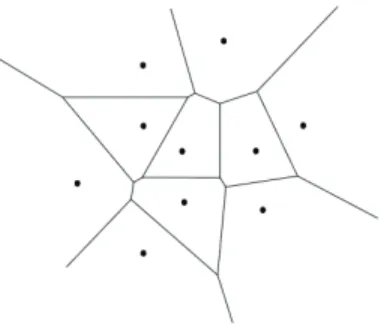
2.1 Voronoi tessellation
Voronoi tessellation is used for modelling proximity problems (Figure 3). The Voronoi tessellation of a set of sites S = {s1, . . . , sn} in d partitions space into n
regions - one for each site - such that the region for a site si consists of all points that are closer to si than to any other site sj S. The set of points that are closest to a particular site si forms the so-called Voronoi cell of si, and is denoted by V (si). Thus, when S is a set of sites in the plane we have
V (si) = {p 2 : dist(p, si) < dist(p, sj) for all ji},
where dist(., .) denotes the Euclidean distance (Berg & Speckmann, 2005).
2.2 Spatial analysis
Spatial analysis is defined as the manipulation of spatial data into different forms in order to extract additional meaning. The major concerns are to investigate the patterns in spatial data and to discover possible relationships between such patterns and other attributes within the study region (Lo & Yeung, 2007). Detailed descriptions of relevant spatial analysis techniques such as buffering and overlaying can be found in de Smith et al. (2009), Lloyd (2009) and O’Sullivan and Unwin (2009).
2.3 Multicriteria decision making (MCDM)
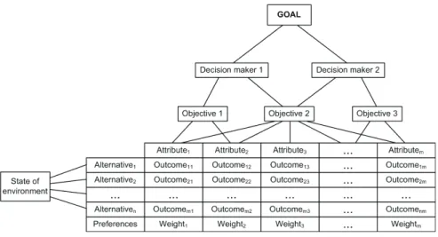
MCDM is generally defined as a decision aid and a mathematical tool allowing the comparison of different alternatives or scenarios according to many criteria, often conflicting, in order to guide the decision maker toward a judicious choice (Chakhar & Mousseau, 2008). In general, MCDM problems involve six components (Malczewski, 1999): a. goal or a set of goals the decision maker attempts to achieve, b. the decision maker or group of decision makers involved in the decision-making process along with their preferences with respect to evaluation criteria, c. a set of evaluation criteria (objectives and/or attributes) on the basis of which the decision makers evaluate alternative courses of action, d. the set of decision alternatives, that decision or action variables, e. the set of uncontrollable variables or states of nature (decision environment), f. the set of outcomes or consequences associated with each alternative-attribute pair. The relationship between the elements of MCDM is shown in Figure 4.
The evaluation of alternatives may be expressed according to different scales (ordinal, interval, ratio). However, a large number of multicriteria methods require that all the criteria are expressed in a similar scale. Standardising the criteria permits the rescaling of all the evaluation dimensions between 0 and 1. This allows between and within criteria comparisons (Chakhar & Mousseau, 2008). Benefit and cost criteria are standardised as follows:
⁄ (benefit criterion) (1)
⁄ (cost criterion) (2)
where is ith raw criterion, is ith standardised criterion (i = 1, 2, …, n).
Following standardisation, a weight ( ) is assigned to each criteria to
reflect their relative importance or priorities usually by normalising them so that
they sum to 1 (∑wi = 1). Decision criteria can then be combined in many ways to
calculate the score ( ). Weighted linear combination is the simplest and widely used method for this purpose (Malczewski, 1999; Carver, 2008; Drobne & Lisec, 2009):
∑ (3)
3. METHODOLOGY
It is essential for automated displacement to find answers to where, when, which objects and how much it will be applied regarding the variety of spatial configurations. The proposed methodology provides answers for those questions.
3.1 Where and when to displace buildings?
3.1.1 Generalisation zones (Where?)
in generalisation decisions (Figure 5). It restricts where buildings of a cluster can be moved. Updating of the zones can be required owing to PAT if a building is eliminated.
Figure 5 - Block, zones and buildings.
3.1.2 Displacement necessity and feasibility (When?)
After individual generalisation and typification of buildings, generalisation zones are analysed with respect to displacement necessity and feasibility. Displacement is necessary if there is minimum distance conflict between buildings within a zone, or a building and its zone intersect with each other. Displacement is feasible if the zone density is smaller than threshold density. Generalisation zone density is calculated dividing the total area of half-MDT-size buffers(MDT-bfs) of the buildings (i.e. 0.1 mm at target scale) by the area of modified generalisation zone, i.e. half-MDT-size clipped version of the initial generalisation zone. Theoretically, a density around 100% means that buildings can be located at the generalisation zone without the legibility conflict. However, this ratio should be smaller in most cases since specific configurations of buildings and specific shapes of the zones can prevent locating the buildings in the zone without conflict. Hence threshold density is calculated using following equation:
where , , is the ratio of the standard distance of generalisation zone vertices
, to the weighted standard distance of buildings , , , MDT is
total area of half-MDT-bf of a building and , is average area of buildings.
Standard distance is calculated using the coordinates ( , ) and the number ( ) of the vertices, the centre of gravity (CoG) of the generalisation zone ( , ) (Equation 6) as well as the initial location ( , , , ) and the average location of buildings weighted by area ( ) (Equation 7). , , , which gives a hint about the feasibility of displacement, is calculated as follows (except , , if , ):
, ½ ½ (5)
, , , ∑ , , ∑
½
(6)
, , , ⁄ , (7)
3.2 Displacement controls and decisions
Candidates (which buildings) and quantities (how much) of displacement are mainly determined through the following criteria (i.e. displacement controls) in generalisation zones:
Ratio of the areas of a Voronoi space and a building , , : It is the weighted total area of Voronoi polygons (i.e the parts in the buffer) within
PAT-bf of a building divided by its area. This criterion is important to understand the approximate size of the empty space that can be allocated to a building.
Displacement distance , : It is the distance between the CoGs of a building and its Voronoi space. This distance is diminished at the same direction if the absolute location change has exceeded the PAT or the some part of building geometry has been outside of its zone after the trial with the temporary copy of the building geometry.
Location change ( ): It is the distance between the previous and the last locations of a building.
Distribution distance change ( ): It is the difference between the distance between the initial CoG of a building and the initial average locations of the building group, and the final CoG of a building and the hypothetical mean location of the building group.
Distribution angle change ( ): It is the angular difference (from the x-axis) between the initial and the last CoGs of a building, and the final CoG of a building and the hypothetical mean location of the building group.
Number of previous displacements ( ): Previous displacements of a building is important to prevent successive displacements of same building that can lead to similar displacement vectors since the locations of other buildings have no changes.
Normalised values of these criteria are calculated for each building in each iteration and the overall score are found by the weighted sum (weighted linear combination). First three criteria have positive effect (benefit) while the others have negative effect (cost) on the overall score (Figure 6). The building with highest score is chosen as displacement candidate if the condition mentioned below is met.
Figure 6 - A framework for MCDM in building displacement.
as a result of empirical tests. If this is the case then another building is chosen as the candidate according to the highness of its weight.
3.3 Displacement strategy
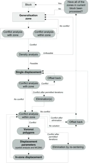
Displacement is applied in generalisation zones of blocks if necessary and feasible (Figure 7).
Displacement trials start with single displacement (see 3.3.1). After all buildings are moved inside the zone via single displacement and failed ones (i.e. not entirely within the zone) are eliminated, minimum distances between buildings are analysed. If there is conflict then in-zone displacement is iteratively applied to candidate buildings. Empirically determined number of iterations permitted in each trial is fifteen times of the current number of buildings except too many small displacement distances (< 0.1 m) in successive and non-successive iterations, which must not exceed two and six times of the number of buildings respectively. In each iteration, Voronoi polygons are created in the zone (see 3.3.2) and displacement controls are calculated mainly by means of Voronoi polygons and spatial analysis. Candidate building is determined according to the score calculated through MCDM (see 3.3.3). In case of failure, new displacement trial is performed again after elimination by re-centering (see 3.3.4). The trials stop if there is a solution or it is accessed to the elimination limit which is one building for every four buildings.
Minimum distance conflicts between buildings and roads or built-up areas are resolved by displacing buildings inside the zone. Positional accuracy is guaranteed by means of the PAT-bf and absolute location change control. Spatial patterns and relationships are imposed by generalisation zone explicitly and the some generalisation controls mentioned above implicitly. Clearly speaking, the zones provide a proper share of map space in the block while some generalisation controls have some effect on the relationships of buildings in the zone since how less they are violated so greater effect they have on the overall score in each iteration
3.3.1 Single displacement
Single displacement individually displaces outside buildings into the zone. New location of a building is determined with one of the following ways (in order of precedence):
a. the CoG of the polygon ( , , , , , ) obtained from the intersection of the generalisation zone with the PAT-bf of the building;
b. the modified CoG from the previous step as seen in Equation (8) and Equation (9), which makes new location closer to the CoG of the zone;
, , , , , , . / (8)
, , , , , , . / (9)
d. the CoG of the polygon obtained from the intersection of the generalisation zone with the MDT-bf of the building;
e. the average value of the CoG of the intersection polygon of the generalisation zone with the PAT-bf of the building and the coordinates of furthest point on the contour of this polygon to the CoG of the building.
Single displacement is performed in the direction of the vector calculated with one of the above-mentioned ways and stops as soon as the building is entirely within the zone. The options are tried sequentially after the buildings are offset back to their initial locations each time if previous one fails. If it is not possible to displace the building inside the zone, it is deleted if at least one building remains.
3.3.2 Creating Voronoi polygons of buildings
Voronoi polygons of the buildings are created so as to approximately calculate the space that can be allocated to them in the zone (Basaraner and Selcuk, 2008). Some extra points on the edges of buildings and the PAT-bf of the generalisation zone are temporarily interpolated for more precise partitioning in the zone. The interpolation distances are 12.5 m (0.25 mm at 1:50 000) for smallest square buildings and 25 m (0.5 mm at 1:50 000) for the other buildings and the PAT-bf. The resulting polygons are clipped by generalisation zone geometry.
3.3.3 Obtaining displacement parameters
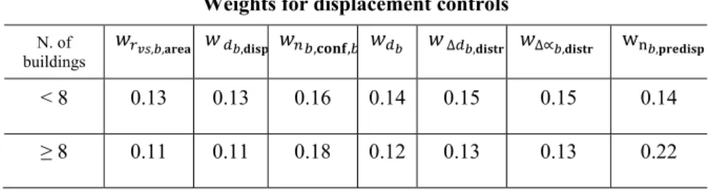
In this phase, displacement decisions (i.e. displacement candidate and quantity) are made in each iteration. Weights of relative importance are assigned to displacement controls regarding the number of buildings (Table 1).
Table 1. Weights for the displacement controls
Weights for displacement controls
N. of
buildings , , , , , ∆ , ∆ ,
w ,
< 8 0.13 0.13 0.16 0.14 0.15 0.15 0.14
≥ 8 0.11 0.11 0.18 0.12 0.13 0.13 0.22
CoGs of the buildings and the zone ( , as well as the iteration number of displacement ( (Equation 10). If the contours of a zone and a Voronoi polygon are touching each other, the weight is increased (Equation 11).
,
⁄
⁄ ⁄ (10)
⁄
(11)
1. The weighted average location of Voronoi polygons ( , , , ) is calculated through the location ( , ), the area ( ) and the weight ( ) of each Voronoi polygon.
, (12)
, (13)
Displacement vector ∆ , , ∆ , is calculated through these coordinates and current location of building. In order to obtain distribution vector ( , , , ) and distribution angle ( , ) as well as distribution distance change (∆ , ) and distribution angle change (∆ , ), hypothetical mean location of buildings ( , , , ) is calculated through initial average location of buildings ( , , , , , ) and the CoG of the zone ( , ):
, . 5 , , .75 (14)
, . 5 , , .75 (15)
The ratio of the areas of a Voronoi space and a building ( , , ) is calculated as follows:
2. Then the number of conflicts of the building with other buildings ( , ) is found. Finally the score , is calculated for the building with the normalised values of displacement controls:
, , , , , , ∆ , , , , ,
∆ , ∆ , ∆ , ∆ , (17)
, ,
If , . and , . then , , (18)
3. A building with the greatest score is selected as displacement candidate, except two cases: a. if same building has been candidate in the last iteration for the zones with four or less buildings, the one with second greatest score is selected as displacement candidate, b. if same building has at least once been candidate in last two iterations for the zones with more than four buildings, the one with third greatest score is selected as displacement candidate.
3.3.4 Elimination by re-centering
3.4 Quantitative analysis of spatial constraints and qualitative evaluation of displacement results
The satisfaction of the spatial constraints of buildings is analysed by zone-based comparison of source (1:25 000) and target data (1:50 000) (Table 2).
Table 2. Conditions of qualitative evaluation.
IF , , = 0 OR , , THEN Evaluation = “Unnecessary” (i.e. no conflict) ELSE IF ≥ THEN Evaluation = “Unfeasible” (i.e. high density) ELSE IF , , > 0 OR , , > 0 THEN Evaluation = “Failed”
(i.e. unresolved conflicts) ELSE IF , = 1 THEN begin
IF , ≤ MDT THEN Evaluation = “Very Good” ELSE IF , ≤ PAT THEN Evaluation = “Good”
ELSE IF , ≤ PAT + MDT THEN Evaluation = “Average” ELSE Evaluation = “Bad”
end ELSE begin
IF , ≤ MDT AND ∆ , , ≤ MDT
AND ∆ , , ≤ 18 THEN Evaluation = “Very Good” ELSE IF , ≤ PAT AND ∆ , , ≤ PAT AND ∆ , , ≤ 45 THEN Evaluation = “Good” ELSE IF , ≤ PAT AND ∆ , , > 45 THEN begin
IF , = , THEN Evaluation = “Average” ELSE
begin
IF ∆ , , ≤ 70 THEN Evaluation = “Good” IF ∆ , , > 70 AND ∆ , , ≤ 80 THEN Evaluation = “Average”
ELSE Evaluation = “Bad” end
end
A qualitative evaluation is made through the quantitative comparison between source and target data. Threshold values are obtained from graphic limits, positional accuracy and the visual examination of cartographic results. In case of 1:1 relation, initial locations of buildings at 1:50 000 are same as of buildings at 1:25 000, but in case of n: m relation (n > m, m > 0), buildings created at average locations during typification substitute for source buildings. MDT is enforced between buildings, between buildings and roads and between buildings and built-up areas. The conflict of a building with surrounding roads or built-up areas is resolved by moving it inside the zone. Average location change (i.e. average positional accuracy) should not exceed PAT. Spatial patterns and relationships are rather difficult to measure. Generalisation zones help to preserve them by reasonable allocation of map space in the blocks. In addition, average distribution distance and angle are used to analyse them locally. Average distribution distance change should not exceed PAT. Threshold values for average distribution angle change are dependent on the number of buildings in the zone. More detailed examination of the evaluation of map generalisation can be found in Bard (2004) and Mackaness and Ruas (2007).
4. EXPERIMENT
4.1 Data, software and hardware
Source dataset is 1:25 000 topographic map. LULLTM programming language is used to develop an interface in Gothic LAMPS2TM, an object-oriented GIS and map production software of 1SpatialTM. Experiment is performed with a notebook with Intel® Centrino CoreTM 2 Duo P8600 2.40 GHz CPU, 3 GB RAM and 256 MB graphic card memory.
4.2 Implementation
Data schema was prepared for buildings within Gothic LAMPS2TM. The experiment was then performed with a displacement menu in a generalisation interface to displace the buildings from 1:25 000 to 1:50 000 (Figure 8).
4.3 Obtained results
Quantitative and graphic results belonging to generalisation zones are given in Appendix. Figure 9 demonstrates the total results of qualitative evaluation and the success rate of displacement excluding the zones where displacement is unfeasible or unnecessary. Total area of the zones is 274034.06 sq m, total number of processed buildings is 155, total processing time is 6 min 50.17 sec and average processing times per zone and building are 6.31 sec and 2.63 sec respectively.
5. DISCUSSION
Following points should be regarded relating to the displacement method:
Generalisation zones are created based on the building clusters in the blocks and updated after typification or elimination.
Displacement is performed after individual generalisation and typification.
Threshold density differs in the zones with same number of buildings since the map space requirement also depends on building distribution.
Displacement is unfeasible in the zones which have still high density after typification.
The area and the distance to its interacting buildings of a Voronoi polygon are weight factors when calculating new possible location for a building since the greater one will provide more space and the far one is more suitable to resolve the conflicts.
Voronoi polygons adjacent to the boundary of its generalisation zone are assigned more weight to be able to more effectively use the map space in the zone.
The weights of Voronoi polygons increase with the iteration number to increase the effect of their size.
Hypothetical mean location is calculated by assuming mean location of final buildings will be close to the CoG of the zone.
All displacement controls have some effects on displacement results and in some cases a solution may not be produced although there is empty space.
The weights for displacement controls are based on experiments and together with the increase in the number of buildings the weight for the number of previous displacement is significantly increased to be able propagate displacement to all buildings.
Generalisation zones are created before contextual generalisation and their final geometries can change depending on the final building set.
If the displacement distance of a building is too small then it is assigned as the score of the building for decreasing its possibility of being displacement candidate to prevent too small displacement.
In case of too much small displacement vectors, the iteration stops and a new trial starts after removal of a building.
The shapes of generalisation zones and the distribution of buildings can make it difficult to find an acceptable solution especially the number of buildings is high.
The zones with “Bad”, “Average” or “Failed” evaluations usually need small corrections to be acceptable.
Displacement is applied in the zones not in the blocks and this provides more local generalisation decisions and hence the displacement success will increase.
A qualitative evaluation is proposed based on quantitative and graphic results and gives a general idea of displacement success.
Multiple criteria (i.e. displacement controls) are combined for determining the candidate building in each iteration to find a compromise between these conflicting criteria.
Voronoi tessellation helps share map space optimally by buildings in the zone and calculate displacement vector.
Generalisation zone density enables to find the zones where displacement is unfeasible.
The method is relatively simple -not based on complex mathematical methods- and can easily be implemented in any GIS software.
Limitations of the method are as follows:
Minimum distance between the buildings in neighbouring zones is not controlled so there can be some conflicts after displacement. This can be resolved either by typification or elimination by re-centering of the conflicted buildings or re-applying displacement after combining the related zones.
Any failure in single displacement can affect displacement results. For instance, the elimination of the buildings located at the narrow sides of the neighbouring zones.
The weights for displacement controls are static.
Elimination during in-zone generalisation can sometimes not succeed in removing the most appropriate building in terms of potential displacement success.
Displacement stops as soon as the minimum distance conflicts are resolved. Spatial patterns and relationships do not have direct effect on finishing the process.
More sophisticated spatial pattern recognition techniques for buildings can improve the displacement operation.
The proposed displacement method differs from the previous works from several points:
Displacement is applied locally by means of generalisation zones from contextual generalisation perspective. To be clear, displacement is only performed in the feasible zones if necessary.
Multiple conflicting criteria are proposed to control the displacement and MCDM contributes to displacement decisions.
Voronoi tessellation is used by weighting to allocate map space to the buildings in the zone.
6. CONCLUSIONS
An iterative displacement method is proposed that can be employed in cartographic generalisation of buildings. It is based on the collective use of Voronoi tessellation, spatial analysis and MCDM. Generalisation zones are created by means of Voronoi tessellation and some spatial analysis techniques such as buffering and overlaying in order to limit the area where building clusters are generalised. Displacement feasibility of a zone is determined by comparing zone and threshold densities. Displacement consists of two steps: Single displacement, i.e. moving the buildings into their zone and in-zone displacement, i.e. conflict resolution between buildings in the zone. Displacement decisions are mainly made with multiple criteria (i.e. displacement controls) in the zones. The values of the criteria are obtained through spatial analysis and Voronoi tessellation. Besides, simple linear weighting approach of MCDM is used to calculate the scores of buildings to find the candidate to displace in each iteration. Minimum distance, positional accuracy and spatial patterns and relationships are three constraints that should be obeyed in displacement. Minimum distance is main triggering and halting criteria of displacement. Minimum distance conflicts between buildings and roads or built-up areas are resolved by single displacement. Minimum distance between buildings is controlled by the MDT-bf. Positional accuracy is guaranteed by the PAT-bf of the building and location change control. Generalisation zones partition the blocks into smaller units for building clusters, which help preserve the spatial patterns and relationships in some degree. The other two implicit criteria are distribution distance change and distribution angle change. The quantitative results show that these values are largely correlated with the graphic results. Future works are to develop more advanced techniques for extracting and preserving spatial patterns and relationships as well as to use dynamic weights for displacement controls in each iteration that may depend on constraints’ violations. In addition interaction between zones ought to be addressed and elimination decisions can be improved.
ACKNOWLEDGEMENTS
REFERENCES
AGENT CONS. Strategic Algorithms Using Organisations. Report D D3. The AGENT Project, ESPRIT/LTR/24939, 2001. Available from: http://agent.ign.fr/deliverable/DD3.pdf, [Accessed: 12.03.2010]
AI, T.; OOSTREOM, P. VAN. Displacement methods based on field analysis. In:
Proceedings of Joint Workshop on Multi-Scale Representations of Spatial Data, Ottawa, Canada: ISPRS WG IV/3, ICA Commission on Map Generalisation, 2002.
BADER, M.; BARRAULT, M.; WEIBEL, R. Building displacement over a ductile truss. International Journal of Geographical Information Science, 19 (8-9), 915-936, 2005.
BARD S. Quality assessment of cartographic generalisation. Transactions in GIS, 8(1), 63-81, 2004.
BASARANER, M.; SELCUK, M. A structure recognition technique in contextual generalisation of buildings and built-up areas. The Cartographic Journal, 48(4), 274-285, 2008.
BERG, M. DE; SPECKMANN, B. Computational geometry: fundamental structures. In: D.P. MEHTA; S. SAHNI (Eds.). Handbook of Data Structures and Applications. Chapman & Hall/CRC Computer & Information Science Series 4, Boca Raton: CRC Press, 62, 1-20, 2005.
BURGHARDT, D.; SCHMID, S. Constraint-based evaluation of automated and manual generalised topographic maps. In: Gartner, G.; F. Ortag, eds.
Cartography in Central and Eastern Europe: Selected Papers of the 1st ICA Symposium on Cartography in Central and Eastern Europe. Lecture Notes in Geoinformation and Cartography. Berlin: Springer, 147-162, 2010.
CARVER, S.J. Multicriteria evaluation. In: K.K. Kemp, ed., Encyclopedia of Geographic Information Science. Thousand Oaks: SAGE Publications, 290-293, 2008.
CHAKHAR, S.; MOUSSEAU, V. Spatial multicriteria decision making. In: S. Shekhar and H. Xiong, eds., Encyclopedia of GIS. New York: Springer, 747-753, 2008.
DANA, P.H. National map accuracy standards (NMAS). In: K.K., Kemp, ed.,
Encyclopedia of Geographic Information Science. Thousand Oaks: SAGE Publications, 304-305, 2008.
DROBNE, S.; LISEC, A. Multi-attribute decision analysis in GIS: weighted linear combination and ordered weighted averaging. Informatica, 33(4), 459-474, 2009.
HARRIE, L. The constraint method for solving spatial conflicts in cartographic generalization. Cartography and Geographic Information Science, 26(1), 55-69, 1999.
HOJHOLT, P. Solving space conflicts in map generalization: using a finite element method. Cartography and Geographic Information Science, 27(1), 65-74, 2000.
LI, Z. Algorithmic Foundation of Multi-Scale Spatial Representation. Boca Raton: CRC Press, 2007.
LLOYD, C.D. Spatial Data Analysis: An Introduction for GIS Users. 1th ed. Oxford: Oxford University Press, 2009.
LONERGAN, M.; JONES, C.B. An iterative displacement method for conflict resolution in map generalization, Algorithmica, 30(2), 287-301, 2001.
MACKANESS, W.A. An algorithm for conflict identification and feature displacement in automated map generalization, Cartography and Geographic Information Systems, 21(4),219-232, 1994.
MACKANESS, W.A.; PURVES, R. Issues and solutions to displacement in map generalisation. In: Proceedings of 19th International Cartographic Conference. International Cartographic Association (ICA), Ottawa, 1081-1090, 1999.
MACKANESS , W.A.; PURVES, R. Automated displacement for large numbers of discrete map objects. Algorithmica, 30(2), 302-311, 2001.
MACKANESS, W.A.; RUAS, A. Evaluation in the map generalisation process. In: W.A. Mackaness; A. Ruas; L.T. Sarjakoski, eds. Generalisation of Geographic Information: Cartographic Modelling and Applications. Oxford: Elsevier, 37-66, 2007.
MALCZEWSKI, J. GIS and multicriteria decision analysis. New York: Wiley, 1999.
REGNAULD, N.; MCMASTER, R. A synoptic view of generalisation operators. In: W.A. Mackaness; A. Ruas; L.T. Sarjakoski, eds. Generalisation of Geographic Information: Cartographic Modelling and Applications. Oxford: Elsevier, 37-66, 2007.
O’SULLIVAN, D.; UNWIN, D. Geographic Information Analysis. Hoboken: Wiley, 2009.
RUAS, A. A method for building displacement in automated map generalisation.
International Journal of Geographic Information Science, 12(8), 789-803, 1998.
SESTER, M. Generalization based on least squares adjustment, In: Proceedings of International Archives of Photogrammetry and Remote Sensing, 33, 931-938, 2000.
SESTER, M. Optimizing approaches for generalization and data abstraction.
International Journal of Geographic Information Science, 19(8-9), 871-897, 2005.
WARE, J.M.; JONES, C.B. Conflict reduction in map generalization using iterative improvement. GeoInformatica, 2(4), 383-407, 1998.
WEIBEL, R.; DUTTON, G. Generalizing spatial data and dealing with multiple representations. In: P. Longley; M.F. Goodchild; D.J. Maguire; D.W. Rhind, eds., Geographical Information Systems: Principles, Techniques, Management and Applications, 2nd edition, vol. 1, Chichester: Wiley, 125–155, 1999.
APPENDIX
N
o. , , , , , , , ∆ ,
∆
, ,
Evalu
ation Map image
1 7 6 5 0.68 0.76 6 2 16.67 9.99 59.92 Good
2 5 3 2 0.66 0.87 2 2 35.58 0.84 31.52 Bad
3 1 1 1 0.25 0.93 0 0 0.00 0.00 0.00 Unnec essary
4 1 1 1 0.35 0.93 0 0 0.00 0.00 0.00 Unnec essary
5 1 1 1 0.74 0.93 0 1 15.83 0.00 0.00 Good
1 6 5 4 0.68 0.78 3 2 11.88 2.76 5.85 Good
2 1 1 1 0.52 0.94 0 0 0.57 0.00 0.00 Unnec essary
3 7 6 4 0.74 0.75 4 4 19.80 1.34 45.92 Good
4 5 4 3 0.69 0.82 2 2 28.08 8.68 24.40 Bad
5 3 2 1 0.68 0.91 0 2 28.56 20.21 62.67 Averag e
6 2 2 2 0.61 0.91 1 1 15.63 1.29 15.06 Good
7 3 3 3 0.49 0.87 2 0 1.60 5.75 1.15 Very good
8 3 3 2 0.77 0.88 2 2 14.20 2.71 64.07 Good
9 3 3 2 0.80 0.86 2 3 10.27 7.63 4.63 Good
10 3 3 3 0.57 0.88 2 0 1.85 8.16 5.09 Very good
11 3 3 2 0.66 0.87 2 0 7.80 2.22 10.00 Very good
12 1 1 1 0.74 0.94 0 1 0.06 0.00 0.00 Failed
13 1 1 1 0.79 0.94 0 1 0.94 0.00 0.00 Failed
14 2 1 1 0.50 0.93 0 1 12.5 15.09 90.00 Good
15 1 1 1 0.44 0.93 0 0 0.00 0.00 0.00 Unnec essary
16 1 1 1 0.89 0.93 0 1 15.00 0.00 0.00 Good
1 5 4 3 0.78 0.83 2 3 16.06 1.09 39.56 Good
2 2 1 1 0.47 0.93 0 1 15.83 15.70 90.00 Good
3 9 9 9 1.49 0.63 14 6 0.00 0.00 0.00 Unfeas ible
4 4 2 2 0.6 0.91 0 2 15.18 0.49 0.39 Good
Appendix (Continued)
N
o. , , , , , , , , ∆ , ,
∆
, ,
Evalu
ation Map image
1 4 3 3 0.81 0.86 0 3 0.56 1.41 7.85 Failed
2 9 5 5 0.70 0.78 2 4 15.46 2.40 38.71 Good
3 6 6 6 1.86 0.74 8 5 0.00 0.00 0.00 Unfeas ible
4 3 3 3 0.76 0.87 2 3 18.39 1.85 19.99 Good
5 3 2 1 0.62 0.93 1 1 20.25 15.22 54.28 Good
6 1 1 1 0.71 0.93 0 1 13.33 0.00 0.00 Good
1 4 4 3 0.83 0.84 3 4 18.30 7.69 0.50 Good
2 4 3 2 0.65 0.88 2 2 11.43 1.02 13.74 Good
3 4 4 3 0.76 0.83 3 4 13.47 3.49 1.90 Good
4 3 3 2 0.64 0.88 3 1 17.63 1.30 18.14 Good
5 4 3 2 0.74 0.87 1 2 26.22 1.33 16.44 Bad
6 2 1 1 0.74 0.93 0 1 0.00 16.28 90.00 Failed
7 1 1 1 0.37 0.93 0 0 0.00 0.00 0.00 Unnec essary
8 4 4 4 0.44 0.84 3 0 3.09 14.52 4.88 Good
9 1 1 1 0.25 0.93 0 0 0.00 0.00 0.00 Unnec essary
10 1 1 1 0.24 0.93 0 0 0.00 0.00 0.00 Unnec essary
11 1 1 1 0.71 0.93 0 1 0.00 0.00 0.00 Failed
12 2 2 1 0.68 0.92 1 1 32.92 12.78 90.00 Averag e
13 1 1 1 0.24 0.93 0 0 0.00 0.00 0.00 Unnec essary
14 1 1 1 0.62 0.93 0 1 21.67 0.00 0.00 Good
15 1 1 1 0.28 0.93 0 1 8.56 0.00 0.00 Very good
1 2 2 2 0.62 0.92 1 1 19.92 2.32 18.90 Good
2 1 1 1 0.57 0.93 0 1 10.00 0.00 0.00 Very good
3 1 1 1 1.06 0.93 0 1 0.25 0.00 0.00 Unfeas ible
Appendix (continued)
N o. ,
, ,
, , , ∆ , ∆ , ,
Eval uatio n
Map image 1 4 4 4 1.57 0.84 3 4 0.09 0.04 0.05 Unfeas
ible
2 4 3 2 0.79 0.88 1 3 4.26 0.37 5.22 Very good
3 1 1 1 1.28 0.93 0 1 0.25 0.00 0.00 Unfeas ible
1 7 3 3 0.57 0.87 1 2 14.47 3.78 41.89 Good
2 4 4 4 0.64 0.84 5 3 15.47 10.41 4.88 Good
3 6 3 2 0.79 0.86 1 3 35.94 0.26 69.26 Bad
4 1 1 1 0.64 0.93 0 1 15.83 0.00 0.00 Good
5 1 1 1 0.78 0.93 0 1 0.00 0.00 0.00 Failed
1 3 3 3 0.78 0.88 2 3 18.09 10.56 8.51 Good
2 2 2 2 0.45 0.93 1 0 12.02 10.50 11.85 Good
3 3 3 2 0.85 0.88 2 3 19.89 1.17 62.97 Good
4 2 1 1 0.74 0.93 0 1 21.67 13.01 90.00 Good
5 1 1 1 0.41 0.93 0 1 1.67 0.00 0.00 Very good
6 1 1 1 1.63 0.93 0 1 0.00 0.00 0.00 Unfeas ible
, the number of buildings in source data
, initial number of buildings (before displacement) , final number of buildings (after displacement)
generalisation zone density
threshold density
, , initial number of conflicts among buildings
, , initial number of conflicts between roads and buildings or built-up areas , average location change between source and target data
∆ , , average distribution distance change between source and target data