Two-Dimensional Critical Potts and its Tricritical Shadow
Wolfhard Janke
Institut f¨ur Theoretische Physik, Universit¨at Leipzig, Augustusplatz 10/11, 04109 Leipzig, Germany
and Adriaan M. J. Schakel
Institut f¨ur Theoretische Physik, Freie Universit¨at Berlin, Arnimallee 14, 14195 Berlin, Germany
Received on 11 October, 2005
These notes give examples of how suitably defined geometrical objects encode in their fractal structure ther-mal critical behavior. The emphasis is on the two-dimensional Potts model for which two types of spin clusters can be defined. Whereas the Fortuin-Kasteleyn clusters describe the standard critical behavior, the geometrical clusters describe the tricritical behavior that arises when including vacant sites in the pure Potts model. Other phase transitions that allow for a geometrical description discussed in these notes include the superfluid phase transition and Bose-Einstein condensation.
Keywords: Potts model; Tricritical behavior; Geometrical clusters; Fractal structure
I. INTRODUCTION
The quest for understanding phase transitions in terms of geometrical objects has a long history. One of the earlier ex-amples, due to Onsager, concerns the superfluid phase tran-sition in liquid4He—the so-called λtransition. During the discussion of a paper presented by Gorter, Onsager [1] made the following remark: “As a possible interpretation of the λ-point, we can understand that when the concentration of vor-tices reaches the point where they form a connected tangle throughout the liquid, then the liquid becomes normal.” Feyn-man also worked on this approach and summarized the idea as follows [2]: “The superfluid is pierced through and through with vortex line. We are describing the disorder of Helium I.” This approach focuses on vortex loops, i.e., one-dimensional geometrical objects, which form a fluctuating vortex tangle. As the critical temperatureTλis approached from below, the
vortex loops proliferate and thereby disorder the superfluid state, causing the system to revert to the normal state. The λtransition is thus characterized by a fundamental change in the typical vortex loop size. Whereas in the superfluid phase only a few small loops are present, close toTλ loops of all
sizes appear. The sudden appearance of arbitrarily large geo-metrical objects is reminiscent of what happens in percolation phenomena at the percolation threshold where clusters prolif-erate. Even on an infinite lattice, a percolating cluster can be found spanning the lattice.
A second example, due to Feynman [3], is related to Bose-Einstein condensation. Here, the relevant geometrical objects are worldlines. In the imaginary-time formalism, used to de-scribe quantum systems at finite temperatureT, the time di-mension becomes compactified,t=−iτ, with 0≤τ≤/kBT,
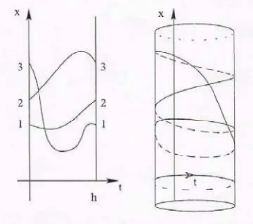
where kB is Boltzmann’s constant. Because of periodic boundary conditions, the worldlines then form closed loops. At high temperatures, where the system behaves more or less classically, the individual particles form separate closed loops wrapping only once around the imaginary time axis. Upon lowering the temperature, these small loops, describing single particles, hook up to form larger exchange rings. A particle in such a composite ring (see Fig. 1) moves in imaginary time
along a trajectory that does not end at its own starting posi-tion, but ends at that of another particle. Hence, although the initial and final configurations are identical, the particles in a composite ring are cyclically permuted and thus become in-distinguishable [3]. Fig. 1 gives an example of three particles, labeled 1, 2, and 3. After wrapping once around the imaginary time axis particle 1 ends at the starting position of particle 2, which in turn ends after one turn around the imaginary time axis at the starting position of particle 3. That particle, finally, ends at the starting position of particle 1. In this way, the three particles are cyclically permuted, forming the cycle(1,2,3). Being part of a single loop which winds three times around the imaginary time axis, the particles cannot be distinguished any longer. At the critical temperature, worldlines prolifer-ate and—again as in percolation phenomena—loops wrapping arbitrary many times around the imaginary time axis appear, signaling the onset of Bose-Einstein condensation [4, 5]. This
FIG. 1: The worldlines of three particles that, after moving a time
0.0
20.0
40.0
60.0
80.0
100.0
0.0
20.0
40.0
60.0
80.0
100.0
0.0
20.0
40.0
60.0
80.0
100.0
0.0
20.0
40.0
60.0
80.0
100.0
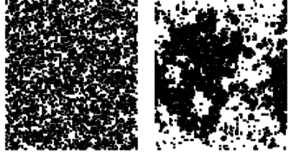
FIG. 2: Snapshots of typical spin configurations of the Ising model on a square lattice of linear sizeL=100 in the normal, hot phase at
β=0.5βc(left panel) and just above the Curie point atβ=0.98βc (right panel). A spin up is denoted by a black square, while a spin down is denoted by a white one.
approach has been turned into a powerful Monte Carlo method by Ceperley and Pollock [6] that can even handle strongly in-teracting systems like superfluid4He (see Ref. [7] for a re-view).
A third example concerns the phase transition in simple magnets. The most elementary model describing such a tran-sition is provided by the Ising model, obtained by assigning a spin that can point either up or down to each lattice site. Fig. 2 shows typical spin configurations for a square lattice in the normal, hot phase and just above the Curie point. For convenience, a spin up is denoted by a black square, while a spin down is denoted by a white one. From these snapshots, the relevant geometrical objects appear to be clusters of near-est neighbor spins in the same spin state (in the following, we will qualify this statement). The normal, disordered phase consists of many small clusters. As the Curie pointTcis ap-proached from above, larger clusters appear, which atTcstart to proliferate—as in percolation phenomena. In the absence of an applied magnetic field, the percolating cluster can con-sist of either up or down spins, both having equal probability to form the majority spin state. Since the percolating spin clusters have a fractal structure, it is tempting to ask whether this structure encodes the standard thermodynamic critical be-havior, as in percolation theory? More generally, we wish to address in these notes the question: Can suitably defined geo-metrical objects encode in their fractal structure the standard critical behavior of the system under consideration? To high-light the basic features, we consider simple models, such as the Ising, the Potts, and the XY model. Moreover, we study them mostly in two dimensions (2D) since many analytical predictions, obtained by using Coulomb gas methods and con-formal field theory, are available there.
The rest of these notes is organized as follows. In the next section, the 2D critical Potts model is discussed. Central to the discussion is the equivalent geometrical representation of this spin model in terms of so-called Fortuin-Kasteleyn clusters [8]. The fractal structure of these stochastic clusters and the way the thermal critical behavior of the Potts model can be
extracted from it are studied in detail. In Sec. III, the tricritical Potts model is discussed. The clusters encoding the tricritical behavior turn out to be the naive clusters of nearest neighbor spins in the same spin state, which feature in Fig. 2. Their fractal structure is connected via a dual map to that of the Fortuin-Kasteleyn clusters, which encode the thermodynamic critical behavior. In Sec. IV, the boundaries of both cluster types are studied. The notes end with a summary of the main results and an outlook to other applications.
II. CRITICAL POTTS MODEL
A. Fortuin-Kasteleyn Representation
The Potts model is one of the well studied spin models in statistical physics [9]. It is defined by considering a lattice with each lattice site given a spin variable si=1,2,· · ·,Q
that can take Q different values. In its standard form, the spins interact only with their nearest neighbors specified by the Hamiltonian
H =−K
∑
i j
δsi,sj−1
, (1)
where K denotes the coupling constant. Nearest neighbor spins notice each other only when both are in the same spin state, as indicated by the Kronecker delta. The Potts model is of particular interest to us as forQ=2 it is equivalent to the Ising model, while in the limitQ→1 it describes ordinary, uncorrelated percolation. The notation∑i jis to indicate that
the double sum over the lattice sites, labeled byiand j, ex-tends over nearest neighbors only. The partition functionZ can be written as
Z=Tr e−βH =Tr
∏
i j
(1−p) +pδsi,sj
, (2)
where β denotes the inverse temperature, and the trace Tr stands for the sum over all possible spin configurations. In writing Eq. (2), use is made of the identity
eβ
δsi,s j−1
= (1−p) +pδsi,sj, (3)
with p=1−e−β, where here and in the sequel we set the coupling constantKto unity. The identity (3) can be pictured as setting bonds with probabilityp/[(1−p) +p] =pbetween two nearest neighbor spins in the same spin state for which δsi,sj=1. When two nearest neighbor spins are not in the same
spin state,δsi,sj=0, then with probability(1−p)/(1−p) =1
the bond is not set, i.e., never. It thus follows, that the partition function can be equivalently written as
ZFK=
∑
{Γ}
pb(1−p)b+a¯ QNC, (4)
specified bybset and ¯bnot set bonds between nearest neigh-bor spins in the same spin state, andapairs of nearest neigh-bor spins not in the same spin state (for which the bonds are never set). Together they add up to the total number of bonds, B=b+b¯+a, so that the exponent ¯b+ain Eq. (4) can also be written asB−b. Only spins connected by set bonds form a cluster. The exponentNCin Eq. (4) denotes the number of clusters, including isolated sites, contained in the bond con-figurationΓ. The factorQNC arises because a given cluster can be in any of theQpossible spin states. Equation (4) is the celebrated Fortuin-Kasteleyn (FK) representation of the Potts model [8]. It gives an equivalent representation of that spin model in terms of FK clusters obtained from the naive geomet-rical clusters of nearest neighbor spins in the same spin state, discussed in the Introduction, by putting bonds with a prob-abilityp=1−e−βbetween nearest neighbors. As geometri-cal clusters are split up in the process, the resulting FK clus-ters are generally smaller and more loosely connected than the geometrical ones.
Not only does the FK representation provide a geometrical description of the phase transition in the Potts model, it also forms the basis of efficient Monte Carlo algorithms by Swend-sen and Wang [10], and by Wolff [11], in which not individual spins are updated, but entire FK clusters. The main advan-tage of the nonlocal cluster update over a local spin update, like Metropolis or heat bath, is that it substantially reduces the critical slowing down near the critical point.
B. FK Clusters
The results of standard percolation theory [12] also apply to FK clusters. In particular, the distributionℓnof FK clusters,
giving the average number density of clusters of massn, takes near the critical point the asymptotic form
ℓn∼n−τe−θn. (5)
The first factor, characterized by the exponentτ, is an entropy factor, measuring the number of ways a cluster of massncan be embedded in the lattice. The second factor is a Boltzmann weight which suppresses large clusters when the parameterθ is finite. Clusters proliferate and percolate the lattice when θtends to zero. The vanishing is characterized by a second exponentσdefined via
θ ∝|T−Tc|1/σ. (6) As in percolation theory [12], the values of the two exponents specifying the cluster distribution uniquely determine the crit-ical exponents. To obtain these relations, we start by consid-ering the radius of gyrationRn,
R2n=
1 n
n
∑
i=1
(xi−x¯)2=
1 2n2
n
∑
i,j=1
(xi−xj)2, (7)
withxithe position vectors of the sites and ¯x= (1/n)∑ni=1xi
the center of mass of the cluster. Asymptotically, the average
Rnscales with the cluster massnas
Rn ∼n1/D, (8)
which defines the Hausdorff, or fractal dimensionD. The av-erage radius of gyrationRngives the typical linear size of
a cluster of massn. A second length scale is provided by the correlation lengthξ, which diverges close toTcwith an expo-nentνasξ∼ |T−Tc|−ν. Both are related via
Rn=ξR(nθ), (9)
whereRis a scaling function, cf. Eq. (5). From the asymptotic behavior (8), the divergence of the correlation length, and the vanishing (6) of the parameterθasTcis approached, the rela-tion
ν= 1
σD (10)
follows, connecting the critical exponentνto the fractal di-mensionDof the clusters andσ.
The fractal dimension can also be related to the entropy ex-ponentτas follows. At criticality, the massnof a cluster is distributed over a volume of typical linear sizeRn, so that
nℓn∼1/Rnd, (11)
withd the dimension of the lattice. This leads to the well-known expression
τ= d
D+1, (12)
in terms of which the correlation length exponent readsν= (τ−1)/dσ.
C. Improved Estimators
To see how physical observables, such as the magnetization mand the magnetic susceptibilityχare represented in terms of FK clusters, we consider the Ising model in the standard notation with the spin variableSi=±1 for simplicity. The
correlation functionSiSjhas a particular simple
representa-tion. When the two spins belong to two different FK clusters
SiSj=
1 4S
∑
i,Sj=±1
SiSj=0, (13)
while when they belong to the same cluster
SiSj=
1 2S
∑
i=Sj=±1
SiSj=1. (14)
That is, ifCidenotes the FK cluster to which the spinSi
be-longs andCjthe one to whichSjbelongs, then
SiSj=δCi,Cj. (15)
For the susceptibility χ≡∑i jSiSj in the normal phase,
Eq. (15) gives
χ=
∑
i j
δCi,Cj=
∑
{C}where the sum∑{C}is over all FK clusters, andnCdenotes the
mass of a given cluster. In terms of the FK cluster distribution
ℓn, the susceptibility can be written as
χ=
∑
n
n2ℓn. (17)
Note that in percolation theory [12], the ratio∑nn2ℓn/∑nnℓn
denotes the average cluster size. Since in the Ising model all Ldspins are part of some FK cluster, we have the constraint
∑
n
nℓn=1. (18)
It thus follows that the right hand of Eq. (17) precisely gives the average size of FK clusters. In other words, this geomet-rical observable directly measures the magnetic susceptibility of the Ising model. From the asymptotic form (5), and the di-vergenceχ∼ |T−Tc|−γof the susceptibility when the critical point is approached, the relationγ= (3−τ)/σ between the critical exponentγand the cluster exponentsσandτfollows.
Also the magnetizationmhas a simple geometrical repre-sentation [12]. In an applied magnetic fieldH, a spin clus-ter of massnChas a probability∝exp(βnCH)to be oriented
along the field direction, and a probability∝exp(−βnCH)to
be oriented against the field direction. The difference between these probabilities gives the magnetizationmCper spin in the
cluster,
mC=tanh(βnCH). (19)
Close to the critical temperature and in the thermody-namic limit L → ∞, the largest cluster dominates, and tanh(βnmaxH)→ ±1 for this cluster, depending on its orien-tation. The magnetization of the entire system (per spin) then becomes
m=±P∞, (20)
whereP∞=nmax/Ld gives the fraction of spins in the largest cluster—the so-called percolation strength. Because of the constraint (18), it is related to the FK cluster distribution via
P∞=1−
∑
n
′
nℓn, (21)
where the prime on the sum indicates that the largest FK spin cluster is to be excluded. The magnetization vanishes near the critical point asm∼ |T−Tc|β. Together with the asymp-totic behavior of the cluster distribution, Eq. (20) with Eq. (21) gives the relationβ= (τ−2)/σ.
These geometrical observables (average cluster size and percolation strength) are calledimproved estimatorsbecause they usually have a smaller standard deviation than the spin observables.
The results just derived for the Ising model also apply to the rest of the critical Potts models [8]. In this way, the thermal critical exponents of these models are completely determined by the exponentsσandτ, characterizing the FK cluster distri-bution. Specifically,
α=2−τ−1
σ , β= τ−2
σ , γ= 3−τ
σ ,
η=2+dτ−3
τ−1, ν= τ−1
dσ , (22)
as in percolation theory [12]. The exponentη, determining the algebraic decay of the correlation function at the critical point, is related to the fractal dimension via
D=1
2(d+2−η). (23)
Consequently
γ/ν=2D−d. (24)
D. Critical Exponents
The critical exponents of the 2DQ-state Potts model are known exactly [13]. It is convenient to parametrize the models as
Q=−2 cos(π/κ¯), (25) with 2≥κ¯≥1. For the Ising model (Q=2) ¯κ=4/3, while for uncorrelated percolation (Q→1) ¯κ=3/2. The correla-tion length exponentνand the exponentη are given in this representation by [13]:
1
ν=yT,1=3− 3
2κ¯, η=2− 1
¯ κ−
3
4κ¯, (26) where yT,1 is the leading thermal exponent. The next-to-leading thermal exponentyT,2readsyT,2=4(1−κ¯), which is negative for ¯κ≥1, implying that the corresponding operator is an irrelevant perturbation. The other critical exponents can be obtained through standard scaling relations. The parameter ¯
κis related to the central chargec, defining the universality class, via [14]
c=1−6(1−κ¯)
2
¯
κ . (27)
Finally, the fractal dimensionD of FK clusters is given by [15, 16]
D=1+ 1
2 ¯κ+ 3
8κ¯, (28)
which givesD=15/8 for the Ising model andD=91/48 for uncorrelated percolation.
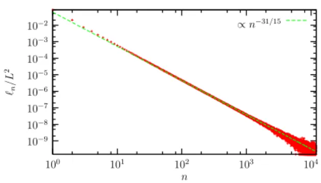
To demonstrate that FK clusters actually percolate at the critical point, Fig. 3 shows the distributionℓnof these clusters
in the 2D Ising model at criticality (θ=0) on a square lat-tice of linear sizeL=512. WithD=15/8, it follows from Eq. (12) that the entropy exponent takes the valueτ=31/15. The straight line, obtained through a one-parameter fit with the slope fixed to the predicted value, shows that asymptot-ically the FK cluster distribution has the expected behavior.
E. Swendsen-Wang Cluster Update
Mass: ∝n −31/15 FK clusters
n ℓn
/L
2
104
103
102
101
100
10−2
10−3
10−4
10−5
10−6
10−7
10−8
10−9
FIG. 3: Distributionℓnnormalized to the volumeL2of FK
clus-ters in the 2D Ising model at criticality on a square lattice of lin-ear sizeL=512. Statistical error bars are omitted from the data points for clarity. The straight line is a one-parameter fit through the data points with (minus) the slope fixed to the predicted value
τ=31/15=2.06666· · ·. The fit illustrates that asymptotically the distribution is algebraic, as expected at criticality.
cluster update [10]. Instead of single spins, entire FK clusters are considered units to be flipped as a whole in this approach. Standard finite-size scaling theory applied to the percolation strengthP∞ and the average cluster sizeχgives the scaling
laws
P∞=L−β/νP(L/ξ), χ=Lγ/νX(L/ξ), (29)
withPandXscaling functions. Precisely atTc, these scaling relations imply an algebraic dependence on the system size L, allowing for a determination of the exponent ratiosβ/ν (see Fig. 4) andγ/ν. Using these geometrical observables as improved estimators for the magnetization and susceptibility, respectively, we arrived at the estimates for the Ising model (Q=2) [17]
β/ν = 0.1248(8)≈1/8,
γ/ν = 1.7505(12)≈7/4, (30) where the right hands give the known values for the Ising critical exponents. These estimates illustrate first of all that FK clusters indeed encode the thermal critical behavior of the Ising model. Moreover, they also illustrate that measuring geometrical observables gives excellent results for the critical exponents. The data were fitted over the rangeL=64−512, using the least-squares Marquardt-Levenberg algorithm.
In Ref. [18], the fractal dimension of FK clusters were ob-tained from analyzing their distribution. This method gives less accurate results than applying finite-size scaling to im-proved estimators. The main problem is related to the fitting window. The fitting range cannot be started at too small clus-ter sizes, where the distribution has not taken on its asymptotic form yet, while too large cluster sizes, which are generated only a few times during a complete Monte Carlo run, are also to be excluded because of the noise in the data and finite-size effects. The results depend sensitively on the precise choice of the fitting window.
FK clusters Geometrical clusters
L P∞
102 101
100
FIG. 4: Log-log plot of the percolation strengthP∞of geometrical and FK clusters at criticality in the 2D Ising model as a function of the linear system sizeL. The straight lines 0.988281L−0.0527for geometrical and 1.00558L−0.1248for FK clusters are obtained from two-parameter fits through the data points. Statistical error bars are smaller than the symbol sizes.
Mass: ∝n
−379/187
Geometical clusters
n
ℓ
G/Ln
2
104
103
102
101
100
10−2
10−3
10−4
10−5
10−6
10−7
10−8
10−9
FIG. 5: DistributionℓG
n normalized to the volumeL2of geometrical
clusters in the 2D Ising model at criticality on a square lattice of linear sizeL=512. Statistical error bars are omitted from the data points for clarity. The straight line is a one-parameter fit through the data points with (minus) the slope fixed to the valueτG=379/187= 2.02673· · ·. The fit illustrates that asymptotically the distribution is algebraic at criticality.
F. Geometrical Clusters
Figure 2 suggests that the geometrical spin clusters also per-colate right at the Curie point of the Ising model. To demon-strate this to be the case, Fig. 5 shows the distribution of these clusters at criticality. Asymptotically, the distribution indeed shows algebraic behavior, implying that clusters of all size appear in the system. It is therefore natural to investigate the exponents associated with the percolation strengthPG
∞ (see
Fig. 4) and the average sizeχGof these geometrical clusters (the superscript “G” refers to geometrical clusters). Using finite-size scaling, as for the FK clusters, we arrived at the estimates [17]
βG/ν = 0.0527(4)≈5/96=0.0520· · ·,
In obtaining these estimates we included percolating clusters. When excluding them, as was done in Ref. [19], the estimates become less accurate [17]. The entropy exponent which fol-lows from these results isτG=379/187, corresponding to the fractal dimensionDG=187/96.
It should be stressed that only in 2D geometrical clusters percolate right at the critical temperature. In higher dimen-sions, geometrical clusters percolate in general too early at a lower temperature, and their fractal structure is unrelated to any thermodynamic singularity.
The 2D exponents (31) are not related to the critical behav-ior of the Ising model and the question arises: What do these exponents describe?
III. TRICRITICAL POTTS MODEL
A. Dual Map
When the pure 2D Potts model is extended to include vacant sites, it displays in addition to critical also tricritical behavior at the same critical temperatureTc[20]. The tricritical ior is known to be intimately connected to the critical behav-ior, and both critical points share the same central charge. To demonstrate this connection, note that for a givenc, Eq. (27) yields two solutions for ¯κ:
¯ κ±=
13−c±
(c−25)(c−1)
12 , (32)
with ¯κ+κ¯−=1, where ¯κ≡κ¯+≥1 and hence ¯κ−≤1. Stated
alternatively, the substitution ¯κ with 1/κ¯ leaves the central charge (27) unchanged,c(κ¯) =c(1/κ¯). When applied to the parametrization (25) of the critical Potts branch, this so-called dual mapyields the parametrization [14]
Qt=−2 cos(π¯κ), (33) of the tricritical branch (the superscript “t” refers to the tri-critical point). Various results for the tri-critical point [13] can be simply transcribed to the tricritical point by using this dual map, leading to [20, 21]
1 νt=y
t T,1=3−
3 2 ¯κ, η
t=2−κ¯− 3
4 ¯κ, (34) while the next-to-leading thermal exponent becomes
ytT,2=4− 4
¯
κ. (35)
To preserve relation (23) under the dual map, the fractal di-mensions of the geometrical and FK clusters must also be re-lated by the map ¯κ→1/κ¯[22, 23]. This gives
DG=1+κ¯
2+ 3
8 ¯κ, (36)
which is indeed the correct fractal dimension of geometrical clusters [24, 25]. In other words, the geometrical clusters can, as far as their scaling behavior is concerned, be considered shadows of the FK clusters. The use of the word “shadow” will become clear when we consider the cluster boundaries in the next section.
B. Ising & itsQt=1Potts Shadow
Equation (36) gives as fractal dimension of the geometrical clusters of the Ising model ( ¯κ=4/3)DG=187/96, implying via Eq. (12)τ=379/187, in accordance with what we found numerically [17]. Note that with ¯κ=4/3, Eq. (33) givesQt=
1. That is, the tricritical model described by the geometrical clusters of the Ising model is the dilutedQt=1 Potts model. Both models share the same central chargec=1/2.
The alert reader may have noticed a curiosity concerning the thermal exponents. According to Eq. (34), the correlation length exponentνttakes the valueνt=1/yt
T,1=8/15 in the dilutedQt=1 Potts model ( ¯κ=4/3). Yet, in our numerical in-vestigation [17] of the geometrical clusters of the Ising model, we seem to observe the correlation length exponentν=1 of the Ising model. Hence,νand not the tricritical exponentνt appears in Eq. (31). In fact, what we see is the tricritical next-to-leading thermal exponent (35), which for the dilutedQt=1 Potts model happens to take the same value as the leading ther-mal exponent of the Ising model,ytT,2=yT,1=1 for ¯κ=4/3.
IV. HULLS & EXTERNAL PERIMETERS
A. FK Clusters
When clusters percolate at a certain threshold, their bound-aries necessarily do too. In the context of uncorrelated per-colation in 2D, external cluster boundaries can be traced out by a biased random walker as follows [26]. The algorithm starts by identifying two endpoints on a given cluster, and putting the random walker at the lower endpoint. The walker is instructed to first attempt to move to its nearest neighbor to the left. If that site is vacant, the walker should try to move straight ahead. If that site is also vacant, the walker should try to move to its right. Finally, if also that site is vacant, the walker is instructed to return to the previous site, to discard the direction already explored, and to investigate the (at most two) remaining directions in the same order. When turning left or right, the walker changes its orientation accordingly. The procedure is repeated iteratively until the upper endpoint is reached. The other half of the boundary is obtained by re-peating the entire algorithm for a random walker instructed to first attempt to move to its right rather than to its left.
For FK clusters, being built from bonds between nearest neighbor sites with their spin in the same spin state, one can imagine two different external boundaries (see Fig. 6). First, one can allow the random walker to move along the FK boundary only via set bonds. This defines thehullof the cluster. Second, one can allow the random walker to move to a nearest neighbor site on the FK boundary irrespective of whether the bond is set or not. This defines theexternal perimeterof the cluster, which is a smoother version of the hull.
a b
FIG. 6: In both panels, a piece of the same single FK cluster of near-est neighbor sites (filled circles) connected by bonds (black links) is shown. Two different external boundaries can be defined: (a) The hull(dark filled circles) is found by allowing a random walker trac-ing out the boundary to move only over set bonds. (b) The exter-nal perimeter(dark filled circles) is found by allowing the random walker to move to a nearest neighbor on the cluster boundary irre-spective of whether the connecting bond is set or not. The external perimeter, which contains two sites less than the hull for this bound-ary segment, is therefore a smoother version of the hull.
B. Fractal Dimensions
The fractal dimensions of the hulls (H) and external perime-ters (EP) of FK clusperime-ters are given by [16, 27, 28]
DH=1+ ¯ κ
2, DEP=1+ 1
2 ¯κ. (37) As for clusters, the average hull and external perimeter sizes diverge at the percolation threshold. LetγHandγEPdenote the corresponding exponents, then because of Eq. (24) withd=2 and Eq. (37)
γH/ν=κ¯, γEP/ν=1/κ¯, (38) where a single correlation length exponentνis assumed.
For illustrating purposes, Fig. 7 shows the distribution of the two boundaries of FK clusters in the Ising model at crit-icality. The straight lines are one-parameter fits through the data points with the slopes fixed to the expected values. Al-though the estimates for DH and DEP we obtained, using finite-size scaling applied to the improved estimators at crit-icality, are compatible with the theoretical conjectures [17], the achieved precision is less than the one we reached for the clusters themselves. The reason for this is as follows. While including percolating clusters when considering the mass of the clusters, we ignore them in tracing out cluster bound-aries. Because of the finite lattice size, large percolating clus-ters have anomalous small (external) boundaries, so that in-cluding them would distort the boundary distributions. More-over, the Grossman-Aharony algorithm [26] used to trace out cluster boundaries generally fails on a percolating cluster as its boundary not necessarily forms a single closed loop any longer. However, as we explicitly demonstrated for the clus-ter mass [17], disregarding percolating clusclus-ters leads to strong corrections to scaling, and therefore to less accurate results.
External perimeters: ∝n −27/11 Hulls: ∝n−
11/5 FK clusters
n ℓn
/L
2
104
103
102
101
100
100
10−2
10−4
10−6
10−8
10−10
10−12
FIG. 7: Distribution normalized to the volumeL2of the hulls and external perimeters of FK clusters in the 2D Ising model at criticality on a square lattice of linear sizeL=512. Statistical error bars are omitted from the data points for clarity. The straight lines are one-parameter fits through the data points with the slopes fixed to the expected values. For clarity, the external perimeters distribution is shifted downward by two decades.
C. Geometrical Clusters
For geometrical clusters, where the bond between nearest neighbor sites with their spin in the same spin state is so to speak always set, hulls and external perimeters cannot be dis-tinguished, and
DGH=DGEP. (39)
The fractal dimension of the boundary is gotten from that of the hull (37) of FK clusters by applying the dual map ¯κ→1/κ,¯ yielding [29]
DGH=1+ 1
2 ¯κ. (40)
Since FK clusters have two boundaries, while geometrical clusters have only one, geometrical clusters have less struc-ture and can be considered shadows of FK clusters under the dual map, as far as their scaling behavior is concerned.
Again for illustrating purposes, Fig. 8 shows the distribu-tion of the hulls of geometrical clusters in the Ising model at criticality. The slow approach to the asymptotic form, with the associated strong corrections to scaling we observed for the hulls of geometrical clusters, stands out clearly from the other distributions. The reason for this is that geometrical clusters have a larger extent than FK clusters. On a finite lattice, perco-lating clusters gulp up smaller ones reached by crossing lattice boundaries. For geometrical clusters this happens more often than for FK clusters, so that disregarding percolating clusters when tracing out cluster boundaries has a more profound ef-fect. In particular, the average hull size is underestimated. With increasing lattice size, the effect becomes smaller, as we checked explicitly [17].
Hulls: ∝n
−27/11
Geometical clusters
n ℓn
/L
2
104
103
102
101
100
100
10−2
10−4
10−6
10−8
10−10
FIG. 8: Distribution normalized to the volumeL2of the hulls of geometrical clusters in the 2D Ising model at criticality on a square lattice of linear sizeL=512. Statistical error bars are omitted from the data points for clarity. The straight line is a one-parameter fit through the data points with the slope fixed to the expected value.
hull was omitted in each measurement, we found corrections to scaling to be virtually absent (see Fig. 11 of that paper). This allowed us to obtain a precise estimate for the fractal di-mension on relatively small lattices.
V. CONCLUSIONS & OUTLOOK
As illustrated in these notes, for the 2D Potts models it is well established that suitably defined geometrical objects en-code in their fractal structure critical behavior. In fact, two types of spin clusters exist, viz., FK and geometrical clusters, which both proliferate precisely at the thermal critical point. As emphasized before, this is special to 2D. In general, geo-metrical clusters percolate at an inverse temperatureβp>βc. The fractal structure of FK clusters encodes the critical ex-ponents of the critical Potts model, while that of geometrical clusters in 2D encodes those of the tricritical Potts model. The fractal structure of the two cluster types as well as the two fixed points are closely related, being connected by the dual map ¯κ→1/κ. This map conserves the central charge, so that¯ both fixed points share the same central charge. The geomet-rical clusters can, as far as scaling properties are concerned, be considered shadows of the FK clusters.
Up to now we considered external boundaries of spin clus-ters as clusclus-ters themselves, which necessarily percolate when the spin clusters do. An alternative way of looking at these boundaries is to consider them as loops. In this approach, it is natural to extend the Ising model in another way and to consider the O(N) spin models, with−2≤N ≤2. The high-temperature (HT) representation of the critical O(N) spin model naturally defines a loop gas, corresponding to a di-agrammatic expansion of the partition function in terms of closed graphs along the bonds on the underlying lattice [30]. The loops percolate right at the critical temperature, and sim-ilar arguments as given in these notes for spin clusters show that the fractal structure of these geometrical objects encode
important information concerning the thermal critical O(N) behavior [31, 32]. This connection was first established by de Gennes [33] for self-avoiding walks, which are described by the O(N) model in the limitN→0. One aspect in which lines differ from spin clusters is that they can be open or closed. It is well known from the work on self-avoiding walks that the loop distribution itself is not sufficient to establish the critical be-havior, as has recently also been emphasized in Ref. [34]. For this, also the total numberzn≡∑jzn(xi,xj)ofopen graphs
ofnsteps starting at xiand ending at an arbitrary sitexj is
needed. Its asymptotic behavior close to the critical tempera-ture, cf. Eq. (5) with Eq. (12),
zn∼nϑ/De−θn, (41)
provides an additional exponentϑ, which together with the loop distribution exponents is needed to specify the full set of critical exponents [32]. In Eq. (41),Ddenotes the fractal dimension of the closed graphs. Note that for spin clusters, the notion of open or closed does not apply, so that the analog of the exponentϑis absent there.
Remarkably, the HT graphs of a given critical O(N) model represent at the same time the hulls of the geometrical clus-ters in theQ-state Potts model with the same central charge [22, 25, 35]. To close the circle, we note that, as in the Potts model, including vacancies in the O(N) model gives rise to also tricritical behavior. The tricritical point corresponds to the point where the HT graphs collapse. In the context of self-avoiding walks (N→0), this point is known as theΘpoint. Using the duality discussed in Sec. III A, we recently conjec-tured that the tricritical HT graphs at the same time represent the hulls of the FK clusters of the Potts model with the same central chargecas the tricritical O(N) model [31]. This con-nection allowed us to predict the magnetic scaling dimension of the O(N)tricritical model, in excellent agreement with re-cent high-precision Monte Carlo data in the range 0≤c0.7 [36].
traced out. When two vortex segments enter a unit cell, it is not clear how to connect them with the two outgoing seg-ments. A popular choice is to randomly connect them, but it might well be that the resulting network is too extended and consequently percolates too early. It is in our mind conceiv-able that a proper prescription for connecting vortex segments could lead to a vortex percolation threshold right at the critical temperature, in the spirit of the FK construction.
As a final remark, we note that even in cases where no ther-modynamic phase transition takes place, the notion of vortex proliferation can be useful in understanding the phase struc-ture of the system under consideration. An example is pro-vided by the 3D Abelian Higgs lattice model with compact gauge field [39]. In addition to vortices, the compact model also features magnetic monopoles as topological defects. It is well established that in the London limit, where the ampli-tude of the Higgs field is frozen, it is always possible to move from the Higgs region into the confined region without en-countering thermodynamic singularities [40]. Nevertheless, the susceptibility data for various observables define a pre-cisely located phase boundary. Namely, for sufficiently large lattices, the maxima of the susceptibilities at the phase
bound-ary do not show any finite-size scaling. Moreover, the suscep-tibility data obtained on different lattice sizes collapse onto single curves without rescaling, indicating that the infinite-volume limit is reached. In Ref. [39] it was argued that this phase boundary marks the location where the vortices prolif-erate. A well-defined and precisely located phase boundary across which geometrical objects proliferate, yet thermody-namic quantities remain nonsingular has become known as a Kert´esz line. Such a line was first introduced in the context of the Ising model in the presence of an applied magnetic field [41].
Acknowledgment
W. J. would like to thank the organisers of this confer-ence for their warm hospitality. A. S. is indebted to Profes-sor H. Kleinert for the kind hospitality at the Freie Universit¨at Berlin. This work was partially supported by the Deutsche Forschungsgemeinschaft (DFG) under grant No. JA 483/17-3 and the EU RTN-Network ‘ENRAGE’:Random Geome-try and Random Matrices: From Quantum Gravity to Econo-physicsunder grant No. MRTN-CT-2004-005616.
[1] L. Onsager, Nuovo Cimento Suppl.6, 249 (1949).
[2] R. P. Feynman, in: Progress in Low Temperature Physics, edited by C. J. Gorter (North-Holland, Amsterdam, 1955), Vol. 1, p. 17.
[3] R. P. Feynman, Phys. Rev.90, 1116 (1953); ibid.91, 1291 (1953);Statistical Mechanics(Benjamin, Reading, 1972). [4] S. Bund and A. M. J. Schakel, Mod. Phys. Lett. B13, 349
(1999).
[5] A. M. J. Schakel, Phys. Rev. E63, 026115 (2001).
[6] D. M. Ceperley and E. L. Pollock, Phys. Rev. Lett.56, 351 (1986).
[7] D. M. Ceperley, Rev. Mod. Phys.67, 279 (1995).
[8] C. M. Fortuin and P. W. Kasteleyn, Physica57, 536 (1972). [9] R. B. Potts, Proc. Camb. Phil. Soc.48, 106 (1952).
[10] R. H. Swendsen and J. S. Wang, Phys. Rev. Lett.58, 86 (1987). [11] U. Wolff, Phys. Rev. Lett.62, 361 (1989).
[12] D. Stauffer and A. Aharony,Introduction to Percolation Theory, 2nd edition (Taylor & Francis, London, 1994).
[13] M. P. M. den Nijs, J. Phys. A12, 1857 (1979); Phys. Rev. B27, 1674 (1983).
[14] J. Cardy, in:Phase Transitions and Critical Phenomena, edited by C. Domb and J. L. Lebowitz (Academic, London, 1987), Vol. 11, p. 55.
[15] H. E. Stanley, J. Phys. A10, L211 (1977). [16] A. Coniglio, Phys. Rev. Lett.62, 3054 (1989).
[17] W. Janke and A. M. J. Schakel, Phys. Rev. E71, 036703 (2005). [18] J. Asikainen, A. Aharony, B. B. Mandelbrot, E. M. Rauch, and
J.-P. Hovi, Eur. Phys. J. B34, 479 (2003). [19] S. Fortunato, Phys. Rev. B66, 054107 (2002).
[20] B. Nienhuis, A. N. Berker, E. K. Riedel, and M. Schick, Phys. Rev. Lett.43, 737 (1979).
[21] B. Nienhuis, J. Phys. A15, 199 (1982); in:Phase Transitions and Critical Phenomena, edited by C. Domb and J. L. Lebowitz
(Academic, London, 1987), Vol. 11, p. 1.
[22] W. Janke and A. M. J. Schakel, Nucl. Phys. B [FS]700, 385 (2004).
[23] Y. Deng, H. W. J. Bl¨ote, and B. Nienhuis, Phys. Rev. E69, 026123 (2004).
[24] A. L. Stella and C. Vanderzande, Phys. Rev. Lett. 62, 1067 (1989).
[25] B. Duplantier and H. Saleur, Phys. Rev. Lett.63, 2536 (1989). [26] T. Grossman and A. Aharony, J. Phys. A19, L745 (1986). [27] H. Saleur and B. Duplantier, Phys. Rev. Lett.58, 2325 (1987). [28] B. Duplantier, Phys. Rev. Lett.84, 1363 (2000).
[29] C. Vanderzande, J. Phys. A25, L75 (1992).
[30] H. E. Stanley,Introduction to Phase Transitions and Critical Phenomena(Oxford University Press, New York, 1971). [31] W. Janke and A. M. J. Schakel, Phys. Rev. Lett.95, 135702
(2005).
[32] W. Janke and A. M. J. Schakel,Anomalous scaling and fractal dimensions, cond-mat/0508734 (2005).
[33] P. G. de Gennes, Phys. Lett. A38, 339 (1972).
[34] N. Prokof’ev and B. Svistunov, cond-mat/0504008 (2005). [35] C. Vanderzande and A. L. Stella, J. Phys. A22, L445 (1989). [36] W. Guo, H. W. J. Bl¨ote, and Y.-Y. Liu, Commun. Theor. Phys.
(Beijing)41, 911 (2004).
[37] E. Bittner, A. Krinner, and W. Janke, Phys. Rev. B72, 094511 (2005).
[38] E. Bittner and W. Janke, Phys. Rev. Lett.89, 130201 (2002); Phys. Rev. B71, 024512 (2005).
[39] S. Wenzel, E. Bittner, W. Janke, A. M. J. Schakel, and A. Schiller, Phys. Rev. Lett.95, 051601 (2005).