STATE FEEDBACK FUZZY-MODEL-BASED CONTROL FOR MARKOVIAN
JUMP NONLINEAR SYSTEMS
Natache S. D. Arrifano
∗ [email protected]Vilma A. Oliveira
∗ [email protected]∗Departamento de Engenharia Elétrica, Universidade de São Paulo, Av. Trabalhador São Carlense, 400
CEP 13566-590, São Carlos, SP, BRASIL
ABSTRACT
This paper deals with the fuzzy-model-based control design for a class of Markovian jump nonlinear systems. A fuzzy system modeling is proposed to represent the dynamics of this class of systems. The structure of the fuzzy system is composed of two levels, a crisp level which describes the Markovian jumps and a fuzzy level which describes the sys-tem nonlinearities. A sufficient condition on the existence of a stochastically stabilizing controller using a Lyapunov function approach is presented. The fuzzy-model-based con-trol design is formulated in terms of a set of linear matrix inequalities. Simulation results for a single-machine infinite-bus power system which is modeled as a Markovian jump nonlinear system in the infinite-bus voltage are presented to illustrate the applicability of the technique.
KEYWORDS: Markovian jump nonlinear systems,
Marko-vian jump fuzzy systems, fuzzy-model-based control, stochastic stabilizability.
RESUMO
Neste artigo, apresentam-se projetos de controladores fuzzy para uma classe de sistemas não-lineares com saltos Marko-vianos. Uma modelagem fuzzy é apresentada para represen-tar esta classe de sistemas na vizinhança de pontos de opera-ção escolhidos. A estrutura do sistema fuzzy é composta de dois níveis, um para descrição dos saltos Markovianos e
ou-Artigo submetido em 28/02/03 1a. Revisão em 15/01/04
Aceito sob recomendação do Ed. Assoc. Prof. Takashi Yoneyama
tro para descrição das não-linearidades no estado do sistema. Uma condição suficiente para a estabilização estocástica do sistema fuzzy considerado é derivada usando uma função de Lyapunov acoplada. O projeto de controle fuzzy é então for-mulado a partir de um conjunto de desigualdades matriciais lineares. Resultados de simulações em um sistema de potên-cia máquina-barramento infinito modelado como um sistema não-linear com saltos Markovianos na tensão do barramento infinito são apresentados para ilustrar a aplicabilidade da téc-nica.
PALAVRAS-CHAVE: Sistemas não-lineares com saltos
Mar-kovianos, sistemas fuzzy com saltos MarMar-kovianos, controle fuzzy, estabilização estocástica.
1
INTRODUCTION
The class of nonlinear systems considered in this paper is a class of hybrid systems, which has different operation modes governed by a Markov process. They are described by a state vector with two components where the first refers to the system modes and the second to the system state. The system modes are represented by a finite-mode Markov pro-cess and the system state in each mode by a system of non-linear differential equations. This class of systems can be used to represent complex real systems, which may experi-ence abrupt changes in their structure and parameters caused by phenomena such as component failures or repairs, chang-ing of subsystem interconnections and abrupt environmental disturbances.
non-linear dynamics, most attention has been given to the lin-ear representation of Markovian jump systems. The Marko-vian jump linear systems (MJLS) were first introduced by Krasovskii and Lidskii (1961) and have been used to model manufacturing management systems, power systems, telecommunication and economic systems (Mariton, 1990). In this context, the linear quadratic control problem was ad-dressed (Boukas and Liu, 2001; Costa et al., 1999; Mariton and Bertrand, 1985a; Mariton and Bertrand, 1985b; Sworder, 1969). Lately, considerable attention has been paid to the ro-bust control, roro-bust stochastic stability and stabilizability of jumping linear uncertain systems (Farias et al., 2000; Boukas et al., 1999; Boukas and Yang, 1999; Costa and Boukas, 1998). In general, the system uncertainties considered ap-pear as norm-bounded uncertainties, which facilitates the ex-tension of the deterministic robust and optimal control tech-niques to the Markovian jump linear systems. Despite this, a more realistic model should consider the nonlinearities of a real system. To the best of our knowledge, the control for Markovian jump nonlinear system (MJNLS) was only con-sidered in Rishel (1975) wherein the optimal control problem is formulated in terms of dynamic programming.
Recently, there have been many successful applications of fuzzy control to nonlinear systems (Arrifano and Oliveira, 2002a; Arrifano and Oliveira, 2002b; Nascimento et al., 2002; Teixeira and ˙Zak, 1999; Tanaka et al., 1998; Wang et al., 1996). In general, the fuzzy control design considers a nonlocal approach which is conceptually simple and straight-forward, where linear feedback control techniques can be used (Wang et al., 1996). To accomplish this, the nonlinear system is represented by a Takagi-Sugeno (TS) fuzzy sys-tem (Takagi and Sugeno, 1985), which is described by fuzzy IF-THEN rules representing local input-output relations of the nonlinear system. The basic idea of this approach is to de-compose the input space into many subspaces, approximat-ing the nonlinear system by a fuzzy blendapproximat-ing of local linear systems associated to each subspace. In fact, it is proved that the TS fuzzy systems are universal approximators (Tanaka and Wang, 2001).
The fuzzy-model based control design uses the so-called par-allel distributed compensation (PDC) scheme and Lyapunov stability. The idea of the PDC scheme is that a linear control is designed for each local linear system. The overall con-troller is again a fuzzy blending of all local linear concon-trollers, which is nonlinear in general. This approach requires a com-mon positive definite matrix that is a solution of all the Lya-punov inequalities built from the local linear systems of the global feedback TS fuzzy system, which are usually formu-lated in terms of linear matrix inequalities (LMI’s) in both the feedback control gain and Lyapunov matrix. However, for a large number of local linear approximations this approach may not provide feasible results because it is not possible to
find a common positive definite Lyapunov matrix as a solu-tion of several Lyapunov inequalities. In order to relax the conservativeness of the stability and stabilization problems, piecewise Lyapunov function approaches have received in-creasing attention (Cao et al., 1997; Cao et al., 1996). With the same purposes, a fuzzy Lyapunov function defined by a fuzzy blending quadratic Lyapunov functions is considered in (Tanaka et al., 2003). The fuzzy Lyapunov function, un-like the piecewise Lyapunov function is smooth.
In this paper, we consider the use of two different fuzzy-model-based control designs for stochastic stabilization of a class of MJNLS. We propose a fuzzy system modeling with two levels of structure, a crisp level which describes the jumps of the Markov process and a fuzzy level which de-scribes the system nonlinearities. Using the state feedback fuzzy system and a coupled Lyapunov function, we formu-late a control design in terms of LMI’s and the stochastic sta-bilizability concept. The remainder of this paper is organized as follows. Section 2 introduces the fuzzy system modeling. Section 3 presents the fuzzy-model-based control. Section 4 deals with the stabilizing fuzzy control design. Simulation results are presented in Section 5 to illustrate the applicability of the proposed approach. Concluding remarks are presented in Section 6.
2
FUZZY SYSTEM MODELING
Consider a class of Markovian jump nonlinear dynamic sys-tems depicted by
˙
x=f(x, u, r); x0=x(0); r0=r(0) (1)
where x ∈ Rn is the system state vector, u ∈ Rm is the control input vector, {r} is a continuous-time Marko-vian process taking values in a finite space state denoted by S = {1,2, ..., N},f(·,·,·)is a smooth nonlinear
func-tion with respect to the first and the second arguments with
f(0,0, .) = 0,x0 andr0are the initial values of the state
and the mode at timet = 0, respectively. The evolution of the stochastic process{r, t≥0}that determines the mode of the system at each timetis assumed to be described by the following transition probability
Pr{r(t+ ∆) =j|r(t) =i}:=
πij∆ +o(∆), i6=j
1−πi∆ +o(∆), i=j (2) where∆ >0,lim∆→0o(∆)∆−1 = 0,πij ≥0is the prob-ability rate between modesiandj, fori 6=j; i, j ∈ Sand
∀i∈S,πi :=−πii =PN
j=1,j6=iπij. A matrixΠ := [πij]is called transition rate matrix. We assume that the Markov pro-cess {r} has stationary distributionµ = (µ1, µ2,· · ·, µN) withµi=P r(r=i)
idea of a switching fuzzy system (SFS) proposed by Tanaka et al. (2000). The SFS have a region rule level which is crisp and a local rule level which is fuzzy. Likewise, the MJFS is structured in upper and lower levels for the modes assumed by the Markov process{r} and for the fuzzy rule in each mode which describes the nonlinearities in the state vectorx, respectively. Thus, theith mode assumed by the MJNLS is represented as follows
Modei:
IfzisMi Then
Rulej:
Ifx1isNij1and . . . andxnisNijn Thenx˙ =Aijx+Biju
i∈S; j= 1,2, . . . , R (3)
wherez ∈ R1 is a mode indicator variable,xanduare as
defined before,Aij andBij are matrices of appropriate di-mensions, which describe local linear representations of the nonlinear system in the vicinity of chosen operation points,
MiandNijk are crisp and fuzzy sets, respectively, andRis the number of inference rules in each mode. In the frame-work of fuzzy systems, the IF-part of the MJFS is referred to as the premise part and the THEN-part is referred to as the consequent part, variablesxandzin the IF-part are known as premise variables. Usually, the premise variables may be functions of state variables, external disturbances, and/or time (Li et al., 2000).
Thus, the MJFS is inferred by a fuzzy blending of the local linear representations (Aij, Bij), i ∈ S, j = 1,2, . . . , R, which are selected according to the mode assumed by the Markov process {r}. Thus, given the triple (x, u, r), the overall fuzzy system is inferred as follows
˙
x = fˆ(x, u, r)
=
N
X
i=1
R
X
j=1
mi(z)nij(x)(Aijx+Biju) (4)
wheremi(z)is the mode indicator which yieldsmi(z) = 1 when r = i, i.e., z ∈ Mi andmi(z) = 0otherwise, and
nij(x)normalized membership functions given by
nij(x) =
Qn
k=1Nijk(xk) PR
l=1 Qn
k=1Nilk(xk)
(5)
withNijk(x) ∈ [0,1]the grade of membership ofxk,k =
1,2, . . . , nin the fuzzy set Nijk. In addition, considering the fact that in (5)Nijk(xk)≥0,j = 1,2, . . . , R, we have
nij(x)≥0andPRj=1nij(x) = 1.
The universe of discourseX:Rn×S→Rnfor the MJFS is given by
X= N∪
i=1Modei=Mode1∪Mode2∪. . .∪ModeN
Modei∩Modeℓ=φ, i6=ℓ, i, ℓ∈S.
Remark 1 The local linear representations of the MJFS can be constructed via the linearization formula proposed by Teixeira and ˙Zak (1999) which yields a good linear ap-proximation of the nonlinear system in the vicinity of a spec-ified operation point even if it is not an equilibrium point.
3
FUZZY-MODEL-BASED CONTROL
The fuzzy-model-based control is in general developed using the PDC scheme. Following this trend, the fuzzy controller proposed here shares the same structure of the MJFS (3) in its premise part, i.e.,
Modei:
IfzisMi Then
Rulej:
Ifx1isNij1and . . . andxnisNijn Thenu=−Fijx
i∈S; j= 1,2, . . . , R (6)
wherez,x,Mi,Nij andRare as defined before andFij ∈
Rm×nare the local feedback gains to be designed. Following
the same lines as in the derivation of the MJFS, we obtain the overall fuzzy controller as
u=− N
X
i=1
R
X
j=1
mi(z)nij(x)Fijx. (7)
In order to obtain the state feedback MJFS as following, we substitute (7) in (4), it results
˙
x =
N
X
i=1
R
X
j=1
mi(z)nij(x) [Aij
− N
X
k=1
R
X
l=1
mk(z)nkl(x)BijKkl
!#
x. (8)
Using the fact thatmi(z)mk(z) = 0,i 6= k, i, k ∈ S, we can write (8) as
˙
x=
N
X
i=1 mi(z)
R
X
j=1
R
X
k=1
nij(x)nik(x)(Aij−BijKik)
x.
Now, using the fact that
R
X
j=1
R
X
k=1
nij(x)nik(x) = R
X
j=1 n2
ij(x) + 2 R
X
j<k
nij(x)nik(x)
andPR
j=1nij(x) = 1, system (9) can be rewritten as
˙ x=
N
X
i=1
mi(z)
R
X
j=1
n2ij(x)Gij+ 2 R
X
j<k
nij(x)nik(x)Hijk
x
withGij :=Aij−BijFij andHijk := 12(Aij −BijFik+ Aik−BikFij),i ∈S,j, k= 1,2, . . . , R. In (10), notation
PR
j<kmeans, for instance forR = 3,
P3
j<kajk ⇔ a12+ a13+a23.
Remark 2 The use of (10) instead of (9) is valuable to re-duce the number of LMI’s conditions in the formulation of the fuzzy control design.
4
STABILIZING FUZZY CONTROL
DESIGN
In this section, we present a sufficient condition for the stochastic stabilization of the MJFS using a coupled Lya-punov function. In order to obtain a systematic fuzzy control design, we formulate the stabilizing control problem in the context of the convex analysis using LMI’s. In the follow-ing, E[·] denotes the expectancy operator andλmin[·] and
λmax[·]denote the minimum and the maximum eigenvalues, respectively.
Definition 1 The MJFS (4) with infinitesimal generatorAis exponentially stable in mean square (ESMS) if there exists a coupled Lyapunov function of the type
V(x, i) =xTPix (10)
∀i ∈ SwithPi := Pr=i a symmetric positive definite con-stant matrix of appropriate dimensions such that
1. V(0, r=i) = 0;
2. V(·,·)is continuous and has bounded first derivatives with respect to the first argument;
3. c1kxk 2
≤V(x, i)≤c2kxk 2
;
4. AV(x, i)≤ −c3kxk 2
;
forc1,c2andc3positive real numbers (Mariton, 1990).
Definition 2 The MJFS (4) is said to be stochastically stable if, for all the initial conditionsx0andr0there exists a state
feedback fuzzy control law (7) satisfying
lim
T→∞E "
Z T
0
x(t, x0, r0, u)Tx(t, x0, r0, u)dt|x0, r0 #
≤xT
0M x0 (11)
for some symmetric positive definite matrixM of appropri-ate dimensions (Ji and Chizeck, 1990).
Proposition 1 The MJFS (4) is stochastically stabilizable with state feedback fuzzy control law (7) if there exist a set of positive definite matricesXiand a set of matricesYijof ap-propriate dimensions satisfying the following LMI’s∀i∈S
Tij Zi
ZT i −Wi
<0;
j= 1,2, . . . , R (12a)
and
Uijk Zi
ZT
i −Wi
<0;
j < k; j, k= 1,2, . . . , R (12b)
where
Tij :=XiATij+AijXi−YijTBijT −BijYij−12πiXi
Uijk:=
XiATij+AijXi−YikTBTij−BijYik
+XiATik+AikXi−YijTBTik−BikYij−12πiXi
Zi:=
h
π1i1/2Xi . . . π
1/2
ii−1Xi π
1/2
ii+1Xi . . . π
1/2
iNXi
i
Wi:=diag X1 . . . Xi−1 Xi+1 . . . XN
Yij:=FijXi Xi:=Pi−1.
Proof: Let mode at timetbei, i.e.,r = i,i ∈ S. In what
follows, for simplicity of notation x denotes the solution
x(t, x0, r0, u) of the MJFS (4) under the initial conditions x0andr0with fuzzy control law (7).
Take the coupled Lyapunov function as in (10). The weak infinitesimal operator of (10) is given by (Ji and Chizeck, 1990)
AV(x, i) := lim
δ→0
1
δ{E[V(x(t+δ), r(t+δ))|x, r=i]
−V(x, r=i)}. (13)
the deterministic derivative. Using Mariton (1990), from (13) it is possible to obtain
AV(x, i) = x˙T ∂
∂xV(x, i) +
N
X
ℓ=1
πiℓV(x, ℓ)
= x˙TPix+xTPix˙+xT N
X
ℓ=1 πiℓPi
!
x.
(14)
Substituting (10) in (14) and using the fact thatmi(z) = 1 whenz∈Mi, we obtain
AV(x, i) = xT
R
X
j=1
n2ij(x)(GijTPi+PiGij)
+2
R
X
j<k
nij(x)nik(x)(HijkT Pi+PiHijk)
x
+xT
N
X
ℓ=1 πiℓPi
!
x (15)
for Gij andHijk as defined before. Now, using the Schur complements (Boyd et al., 1994) and substitutingTij,Uijk,
Zi,Wi,Yij andXi as defined before, LMI’s in (12) can be reduced to
GTijPi+PiGij+ N
X
ℓ=1
πiℓPℓ<0;
j = 1,2, . . . , R (16a)
and
HT
ijkPi+PiHijk+ N
X
ℓ=1
πiℓPℓ<0;
j < k; j, k= 1,2, . . . , R. (16b)
Multiplying (16a) byn2
ij(x)and (16b) by2nij(x)nik(x), we have
R
X
j=1 n2
ij(x)[GTijPi+PiGij]
+
R
X
j=1 n2
ij(x) N
X
ℓ=1
πiℓPℓ<0 (17a)
and
2
R
X
j<k
nij(x)nik(x)[HijkT Pi+PiHijk]
+2
R
X
j<k
nij(x)nik(x) N
X
ℓ=1
πiℓPℓ<0. (17b)
Now, adding (17a) to (17b) and again using the fact that
R
X
j=1
R
X
k=1
nij(x)nik(x) = R
X
j=1 n2
ij(x) + 2 R
X
j<k
nij(x)nik(x)
andPR
j=1nij(x) = 1, we obtainAV(x, i)<0forx6= 0.
Now, defining
L( ¯Gij,H¯ijk, Pi) := ¯GTijPi+PiG¯ij
+2( ¯HT
ijkPi+PiH¯ijk) + N
X
ℓ=1
πiℓPℓ (18)
with G¯ij = PRj=1n 2
ij(x)Gij and H¯ijk = PRj<k
nij(x)nik(x)Hijkand substituting (18) in (15), we obtain
AV(x, i) =xTL( ¯Gij,H¯ijk, Pi)x. (19)
Therefore, we have for allx6= 0andi∈S
AV(x, i)
V(x, i) =
xTL( ¯G
ij,H¯ijk, Pi)x
xTP ix
≤ −ρ (20)
whereρis a positive real number given by
ρ= min
i∈S
λmin
−L( ¯Gij,H¯ijk, Pi)
λmax[Pi]
. (21)
By the Dynkin’s formula (Kushner, 1967), we have
E[V(x(t), r(t))]−V(x0, r0) =E Z t
0
AV(x(s), r(s))ds
.
(22)
Then, substituting (20) in (22), we obtain
E[V(x(t), r(t))]−V(x0, r0)
≤E
Z t
0
−ρV(x(s), r(s))ds
=−ρ
Z t
0
E[V(x(s), r(s))ds]. (23)
Using the Gronwall-Bellman Lemma (Khalil, 1996) in (23), we have
E[V(x(t), r(t))]≤V(x0, r0) exp(−ρt). (24)
it results
lim
T→∞E "
Z T
0 xTP
rxdt|x0, r0 #
≤ 1
ρx
T
0Prx0
≤ 1
ρλmax[Pr]x
T
0x0.
(25)
Considering the fact that in (25)Pris a symmetric positive definite matrix for allr ∈ S, the result follows by
Defini-tions 1 and 2. ✷
4.1
Performance indices in the fuzzy
con-trol design
Like stability, performance indices, such as decay rate and control input, play a key role in the stabilizing fuzzy control design. The speed response of a controlled system is related to decay rate, that is, the largest Lyapunov exponent. In ad-dition, there are some applications in real systems, where the control input has to be limited to guarantee the system oper-ation conditions. In what follows, we formulate the stabiliz-ing fuzzy control design usstabiliz-ing the decay rateαi:=αr=iand control inputγi:γr=i,i∈Sin the context of LMI’s.
Proposition 2 Assume that the decay rateαi >0,i∈ Sis known. The condition
AV(x, i)≤ −2αiV(x, i) (26)
is enforced to all trajectories of the MJFS (4) with state feed-back fuzzy control law (7), if there exist a set of positive definite matricesXiand a set of matricesYij of appropriate dimensions satisfying the following LMI’s∀i∈S
Tij Zi
ZT i −Wi
<−2αi
Xi 0
0 0
;
j= 1,2, . . . , R (27a)
and
Uijk Zi
ZT
i −Wi
<−2αi
Xi 0
0 0
;
j < k; j, k= 1,2, . . . , R (27b)
whereTij,Uijk,Zi,Wi,XiandYijare as defined before.
Proof: The proof follows the same lines of the proof of
Proposition 1. ✷
Proposition 3 Assume that the initial condition x0 is
known. The constraint
E[uTu|x, r=i]≤γi2 (28)
is enforced to all trajectories of the MJFS (4) with state feedback fuzzy control law (7), if the following LMI’s hold
∀i∈S
1 xT
0 x0 Xi
≥0 (29a)
and
Xi YijT
Yij γiI
≥0;
j= 1,2, . . . , R (29b)
whereXiandYijare as defined before.
Proof: Assume thatV(x, i)in (10) is a Lyapunov function for all trajectories of the MJFS (4) with state feedback fuzzy control law (7). Substituting (7) in (28) and using the fact thatmi(z)mℓ(z) = 0,i6=ℓ, i, ℓ∈S, we have
E
R
X
i=1 m2
i(z)
R
X
j=1
R
X
k=1
nij(x)nik(x)xTFijTFijx
≤γ 2
i.
(30)
Let the mode at timetbei, i.e.,r=i,i∈S. Thus, (30) can
be written as
R
X
j=1
R
X
k=1
nij(x)nik(x)xT
1
γ2
i
FijTFij
x≤1. (31)
Now, we use (29a) in order to obtain (31). Using the Schur complements in (29a) and (29b), it results for alli∈S
xT0Pix0≤1 (32a)
and
1
γ2F
T
ijFij−Pi≤0;
j= 1,2, ..., R. (32b)
Multiplying (32b) by nij(x) and using the fact that
PR
j=1nij(x) = 1, we obtain
R
X
j=1
nij(x)xT
1
γ2
i
FijTFij−Pi
x≤0. (33)
It can be shown that (Tanaka and Wang, 2001)
R
X
j=1
R
X
k=1
nij(x)nik(x)xT
1
γ2F
T
ijFij−Pi
x
≤ R
X
j=1
nij(x)xT
1
γ2
i
FT
ijFij−Pi
Thus, using (33) in (34), we have
R
X
j=1
R
X
k=1
nij(x)nik(x)xT
1
γ2F
T
ijFij−Pi
x≤0 (35)
which is the same as
R
X
j=1
R
X
k=1
nij(x)nik(x)xT
1
γ2F
T ijFij
x≤xTP
ix. (36)
Finally, asV(x, i) ≤ xT
0Pix0 by (32a), from (36), we
ob-tain (31) and the result follows. ✷
A stabilizing control design with the decay rate and the con-trol input constraints can be defined as follows: Find a set of positive definite matricesXi and a set of matricesYij of appropriate dimensions satisfying (27) and (29)∀i∈S.
Remark 3 In the approach given, the fuzzy-model-based control design is based on the matrices(Aij, Bij,Π),i∈S,
j = 1,2, . . . , R. Thus, the control design based on LMI’s conditions is strongly related to the number of inference rules and to the modes assumed by the Markov process. The properties of the normalized membership functions can be explored in order to reduce the number of intersections among the fuzzy sets and thus producing more relaxed LMI conditions. Examples of fuzzy-model-based control design using relaxed LMI conditions are given in Teixeira et al. (2003), Teixeira et al. (2000), and Tanaka et al. (1998).
Remark 4 In order to consider the stochastic stabilization of the MJNLS in case the equilibrium point is not the ori-gin, that is, (x, u) 6= 0, one should perform a change of coordinates to make the origin the new equilibrium, before designing the fuzzy control (7) using Propositions 1, 2 and 3.
5
SIMULATION RESULTS
In this section, an illustrative example of the application of the developed approach is given. We consider the same ex-ample as in Guo et al. (2001), a single-machine-infinite-bus (SMIB) power system shown in Figure 1. The dynamic op-eration of the SMIB power system was modeled as being a Markovian jump nonlinear system described by
˙
x1 = x2
˙
x2 = −
D
2Hx2+
ω0
2H(Pm−x3)
˙ x3 =
xds x′
dsT
′
do
"
Tdo′ (xd−x
′
d)
zsin(x1)
xds
2
x2+Pm−x3
#
+cos(x1)
sin(x1)
x2x3+
xds x′
dsT
′
do
zsin(x
1)
xds
kcu
(37)
Figure 1: Single-machine-infinite-bus power system.
Figure 2: Transition modes of the SMIB power system.
where{x, z}is a joint Markov process with stationary distri-butionµ = (0.3, 0.5, 0.2),x1the power angle of the
gen-erator [rad],x2the relative speed of the generator [rad/s],x3
the active power delivered to bus [p.u.],uthe input voltage of the SCR amplifier of the generator [p.u.],z :=Vsthe in-finite bus voltage [p.u.], D the damping constant [p.u.],H
the inertia constant [s],ω0the synchronous machine speed
[rad/s],Pmthe mechanical input power [p.u.],T ′
dothe direct axis transient short-circuit time constant [s],xd,x
′
d,xdsand
x′dsthe system reactances [p.u.]. In the simulations, we adopt the following numerical values of the physical parameters:
D = 5, H = 4, ω0 = 314.159, T
′
do = 6.9, Kc = 1,
xd= 1.8623,x ′
d= 0.257,xds= 2.4753andx ′
ds= 0.8693.
System (37) presents the following equilibrium pointxe =
[2π/5 0 0.9]T andu
e = 0. As mentioned in Remark 4, it is necessary to perform a change of coordinates to bring the equilibrium of the system (37) to the origin. For this purpose, we adoptξ = x−xeandυ = u−ue. Using these new coordinates, we may write (37) as
˙
ξ1 = ξ2
˙
ξ2 = −
D
2Hξ2+
ω0
2H(ξ3+ 0.9)
˙ ξ3 =
xds x′
dsT
′
do
"
Tdo′ (xd−x
′
d)
zsin(ξ1+ 2π/5)
xds
2
ξ2
#
−
xds x′
dsT
′
do
(ξ3+ 0.9) +
cos(ξ1+ 2π/5)
sin(ξ1+ 2π/5)
ξ2(ξ3+ 0.9)
+ xds
x′
dsT
′
do
zsin(ξ1+ 2π/5)
xds
kcυ.
(38)
mode 2: 1.1040 p.u. (normal load) and mode 3: 0.9936 p.u. (heavy load). The transitions among the modes are illustrated in Figure 2. In accordance with the stationary distributionµ
for the Markov processr, we adopt the following transition probability rate matrix forz
Π =
0.1 −0.1 0
−0.06 0.1 −0.04
0 −0.1 0.1
.
In order to obtain the local linear representations of sys-tem (38) in each mode, we adopt R = 2 and consider deviations of ±π/5 in x1, which gives the following
lin-earization pointsx¯: mode 1: x¯R=1 = [π/5 0 1.089]and
¯
xR=2= [3π/5 0 1.089], mode 2:x¯R=1= [π/5 0 0.9]and
¯
xR=2 = [3π/5 0 0.9]and mode 3:x¯R=1= [π/5 0 0.729]
and x¯R=2 = [3π/5 0 0.729]. Thus, using the
pro-cedure given in the Appendix, the following matrices
(Aij, Bij), i = 1,2,3, j = 1,2for the SMIB system are obtained
A11=
0 1.0000 0
0 −0.6250 −39.2699
0 1.8792 −0.4127
;B11=
0 0
0.1190
;
A12=
0 1.0000 0
0 −0.6250 −39.2699
0 0.6418 −0.4127
;B12=
0 0
0.1926
;
A21=
0 1.0000 0
0 −0.6250 −39.2699
0 1.5530 −0.4127
;B21=
0 0
0.1082
;
A22=
0 1.0000 0
0 −0.6250 −39.2699
0 0.5304 −0.4127
;B22=
0 0
0.1750
;
A31=
0 1.0000 0
0 −0.6250 −39.2699
0 1.2580 −0.4127
;B31=
0 0
0.0974
;
A32=
0 1.0000 0
0 −0.6250 −39.2699
0 0.4296 −0.4127
;B32=
0 0
0.1575
.
The mode indicator membership functionsmi(.),i= 1,2,3 are crisp functions which represent the operating modes, in this casemi(z) = 1, ifr=iandmi(z) = 0, otherwise. The normalized membership functionsnij(.),j = 1,2describe the range of the state variablesx1 andx3 in each mode as
shown in Figure 3 and are obtained from standard member-ship functions available in the Fuzzy Logic Toolbox of Mat-lab. A suitable range for the state variables can be determined by constrainingx1in the interval[π/5, 3π/5].
Thus, the fuzzy modeling for the SMIB power system (38) is given by
Mode 1:
Ifzis “1.2144 p.u.”
Then
Rule 1:
Ifx1is “aboutπ/5rad/s” and
x3is “closer to 1.089 p.u.”
Then x˙ =A11x+B11
Rule 2:
If x1is “about3π/5rad/s” and
x3is “far from 1.089 p.u.”
Then x˙ =A12x+B12
Mode 2:
Ifzis “1.1040 p.u.”
Then
Rule 1:
Ifx1is “aboutπ/5rad/s” and
x3is “closer to 0.9 p.u.”
Thenx˙=A21x+B21
Rule 2:
Ifx1is “about 3π/5rad/s” and
x3is “far from 0.9 p.u.”
Thenx˙=A22x+B22
Mode 3:
Ifzis “0.9936 p.u.”
Then
Rule 1:
Ifx1is “aboutπ/5rad/s” and
x3is “closer to 0.729 p.u.”
Thenx˙=A31x+B31
Rule 2:
Ifx1is “about3π/5rad/s” and
x3is “far from 0.729 p.u.”
Thenx˙=A32x+B32.
Therefore, using (Aij, Bij,Π), i = 1,2,3, j = 1,2, we obtain the feedback gains for the stabilization of the SMIB power system (38) by solving the LMI’s in Proposition 1 us-ing the LMI Control Toolbox of Matlab. In order to use per-formance indices in the stabilizing control design, we adopt decay ratesα1 = 5,α2 = 0andα3 = 5and control input
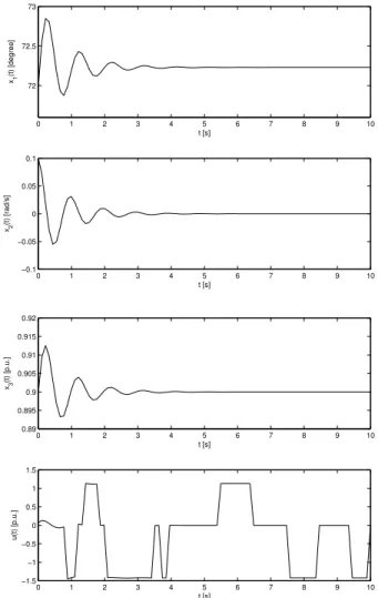
constraintsγi = 6fori= 1,2,3. We take the initial condi-tions asx0= [2π/5 0−0.01 0.9]andr0= 1.1040.
-−1000 0 100 200 0.2
0.4 0.6 0.8 1
x1(t) [degree]
Membership grade
N
111
N
121
−1000 0 100 200 0.2
0.4 0.6 0.8 1
x1(t) [degree]
Membership grade
N
211
N
221
−1000 0 100 200 0.2
0.4 0.6 0.8 1
x1(t) [degree]
Membership grade
N
311
N
321
0 1 2
0 0.2 0.4 0.6 0.8 1
x
3(t) [p.u.]
Membership grade
N
113
N
123
0 1 2
0 0.2 0.4 0.6 0.8 1
x
3(t) [p.u.]
Membership grade
N
213
N
223
0 1 2
0 0.2 0.4 0.6 0.8 1
x
3(t) [p.u.]
Membership grade
N
313
N
323
Mode 1 Mode 2 Mode 3
Figure 3: Membership functions adopted.
0 1 2 3 4 5 6 7 8 9 10
0.95 1 1.05 1.1 1.15 1.2 1.25
z(t) [p.u.]
t [s]
Figure 4: Deviations in the infinite-bus voltagezfollowing the transition rate matrixΠ.
SMIB power system with stabilizing fuzzy control + decay rate + input control constraint. In both cases, we use the soft-ware provided in Waner and Costenoble (2002) to simulate
zwhich is shown in Figure 4 for a period of time. Figures 5 and 6 show the main system responses and Table 1 presents the control design results for both Cases 1 and 2.
The obtained results are comparable to the results presented in Guo et al. (2001). Note that, in both Cases 1 and 2 the system stabilization is satisfactory. In Case 2, the use of con-straints in the stabilizing control design reduces the fluctua-tions in both state variables and control input. The advantage of using Markov jump systems to model the SMIB power system can be clearly seen as we include in the SMIB power system a more refined description of the infinite-bus voltage as compared to that used in Guo et al. (2001). For instance, there, one considers a constant value for the infinite-bus volt-age and the changes in the external load during time are not represented. Taking into account the information on how the
0 1 2 3 4 5 6 7 8 9 10 71.8
71.9 72 72.1 72.2 72.3
x1
(t) [degree]
t [s]
0 1 2 3 4 5 6 7 8 9 10 −0.1
−0.05 0 0.05 0.1
x2
(t) [rad/s]
t [s]
0 1 2 3 4 5 6 7 8 9 10
0.84 0.86 0.88 0.9 0.92 0.94
x3
(t) [p.u.]
t [s]
0 1 2 3 4 5 6 7 8 9 10
−8 −6 −4 −2 0 2 4
u(t) [p.u.]
t [s]
Figure 5: Case 1 - SMIB power system state variables and control.
infinite-bus voltage can vary, we can provide less restrictive conditions for the system stability using controllers with bet-ter performance. Another important point concerns the sta-bility of the SMIB power system. Using the technique pro-posed in Guo et al. (2001), the system must be stable for all deviations in the infinite-bus voltage, whereas in the stochas-tic stability framework, stability of all operation modes is not even required.
6
CONCLUDING REMARKS
Table 1: Control design results.
Mode Case 1
1 F11=
−13.9060 −56.9870 5.2482
F12= − 9.2534 −43.2570 6.5994
2 F21=
−14.5150 −60.7340 6.5752
F22=
− 9.6708 −45.2000 8.0468
3 F31=
−15.3360 −65.5510 8.2105
F32=
−10.2320 −47.8480 9.8305
Mode Case 2
1 F11=
−8.64×10⁻⁹
0.8244 7.7447
F12= 2.02×10⁻⁹ −1.1686 7.1610
2 F21=
−7.58×10⁻⁹
0.7866 7.5597
F22= −5.58×10⁻⁹ −1.0637 6.9946
3 F31=
−4.82×10⁻⁹ 0.6616 6.7462
F32= −5.20×10⁻⁹ −0.8643 6.2894
the nonlinear system complexity and the number of LMI con-ditions is basically a combination of the number of inference rules of the fuzzy system and the number of inference rules of the fuzzy control. The number of inference rules can be re-duced using local approximations of the nonlinear system but stability of the feedback nonlinear system is not guaranteed. In this paper we use local approximations to build the MJFS which represents the class of MJNLS considered. By heuris-tically choosing regions of the subspace that better represent the dynamics of the MJNLS we guarantee the convergence of the solutions reducing the approximation errors.
A fuzzy-model-based control law is used to stabilize the MJFS and then, the stochastic stability and stabilizability concepts are used to formulate the control design in the con-text of LMI’s. The advantage of this approach can be clearly seen, for instance, we could consider in the fuzzy modeling a more refined description of the parameter variations in the nonlinear system. Taking into account this, we give less re-strictive conditions for stability using a coupled Lyapunov function resulting in controllers which provide better perfor-mance.
Another important point concerns the stochastic stability. In comparison with the conventional techniques in the deter-ministic sense, stability of all system modes is not even re-quired. In the proposed approach, whenu= 0, stability in each system mode is given in terms of the matrices (Aij,Π),
i∈S,j = 1,2, . . . , R, that is, stability in each mode is
ver-ified wheneverRe{λ[Aij− 12πiI] <0,πi ≥ 0whereas in
the conventional techniques, stability in each mode is verified only ifRe{λ[Aij]}<0.
Future work include the design of robust fuzzy controllers to consider in the control design the approximation error be-tween the fuzzy-model-based system and the nonlinear
sys-0 1 2 3 4 5 6 7 8 9 10
72 72.5 73
x1
(t) [degree]
t [s]
0 1 2 3 4 5 6 7 8 9 10
−0.1 −0.05 0 0.05 0.1
x2
(t) [rad/s]
t [s]
0 1 2 3 4 5 6 7 8 9 10
0.89 0.895 0.9 0.905 0.91 0.915 0.92
x3
(t) [p.u.]
t [s]
0 1 2 3 4 5 6 7 8 9 10
−1.5 −1 −0.5 0 0.5 1 1.5
u(t) [p.u.]
t [s]
Figure 6: Case 2 - SMIB power system state variables and control.
tem and the development of a dynamic feedback controller to consider incomplete information of the system state.
ACKNOWLEDGMENTS
This work was supported by the Fundação do Amparo à Pesquisa do Estado de São Paulo (FAPESP) under grant 00/05060-1 and by the Conselho Nacional de Desenvolvi-mento Cientifico e Tecnológico under grant 473932/2003-2 Científico e . The authors would like to thank the reviewers for their valuable comments and sugestions
REFERENCES
Arrifano, N. S. D. and Oliveira, V. A. (2002b). Synthe-sis of an LMI-based fuzzy control system with guar-anteed cost performance: a piecewise approach,Proc. XIV Congresso Brasileiro de Automatica, Natal, RN, pp. 2981–2986.
Boukas, E. K. and Liu, Z. K. (2001). Suboptimal design of regulators for jump linear system with time-multiplied quadratic cost, IEEE Transactions on Automatic Con-trol46(1): 944–949.
Boukas, E. K., Liu, Z. K. and Al-Sunni, F. (1999). Guar-anteed cost control of markov jump uncertain system with time-multiplied cost function,Proc. 38th Confer-ence Decision and Control, pp. 4125–4130.
Boukas, E. K. and Yang, H. (1999). Exponential stabilizabil-ity of stochastic systems with markovian jump parame-ters,Automatica35(9): 1437–1441.
Boyd, S., Ghaoui, L. E., Feron, E. and Balakrishnan, V. (1994). Linear matrix inequalities in system and con-trol theory, Philadelphia : SIAM.
Cao, S. G., Rees, N. W. and Feng, G. (1996). Analysis and design of a class of continuous time fuzzy control systems,International Journal of Control64(6): 1069– 1087.
Cao, S. G., Rees, N. W. and Feng, G. (1997). Analysis and design for a class of complex control systems, part ii: Fuzzy controller design,Automatica33(6): 1029–1039.
Costa, O. L. V. and Boukas, E. K. (1998). Necessary and sufficient condition for robust stability and stabilizabil-ity of continuous-time linear systems with markovian jumps, Journal of Optimization Theory and Applica-tions99(2): 359–379.
Costa, O. L. V., do Val, J. B. R. and Geromel, J. C. (1999). Continuous-time state-feedback h2-control of marko-vian jump linear systems via convex analysis, Automat-ica35(2): 259–268.
Farias, D. P., Geromel, J. C., do Val, J. B. R. and Costa, O. L. V. (2000). Output feedback control of markov jump linear systems in continuous-time, IEEE Transactions on Automatic Control45(5): 944–949.
Guo, Y., Hill, D. J. and Wang., Y. (2001). Global tran-sient stability and voltage regulation for power systems, IEEE Transactions on Power Systems16(4): 678–688.
Ji, Y. and Chizeck, H. J. (1990). Controllability, stabi-lizability, and continuous-time markovian jump lin-ear quadratic control,IEEE Transactions on Automatic Control35(7): 777–788.
Khalil, H. (1996).Nonlinear systems, USA: Macmillan Pub-lishing Company.
Krasovskii, N. N. and Lidskii, E. A. (1961). Analytical de-sign of controllers in systems with random attributes I, II, III,Automation Remote Control22: 1021–1025, 1141–1146, 1289–1294.
Kushner, H. J. (1967). Stochastic stability and control, New York: Academic.
Li, J., Wang, O. H., Niemann, D. and Tanaka, K. (2000). Dynamic parallel distributed compensation for Takagi-Sugeno:an LMI approach,Information Sciences123 (3-4): 201–221.
Mariton, M. (1990). Jump linear systems in automatic con-trol, New York: Marcel Dekker.
Mariton, M. and Bertrand, P. (1985a). Output feedback for a class of linear systems with stochastic jumping parameters, IEEE Transactions on Automatic Control
30(9): 898–900.
Mariton, M. and Bertrand, P. (1985b). Robust jump linear quadratic control: a mode stabilizing solution, IEEE Transactions on Automatic Control30(11): 1145–1147.
Nascimento, R. R., Oliveira, V. A., Arrifano, N. S. D., Gesu-aldo, E. and Tosetti, J. P. V. (2002). Control of the molten steel level in a strip-casting process using fuzzy T-S models,Proc. 15th Triennial World Congress of the International Federation of Control,Barcelona,Spain, number 02710.
Rishel, R. (1975). Dynamic programming and minimum principles for systems with jump markov disturbances, SIAM Journal on Control13(2): 338–371.
Sworder, D. D. (1969). Feedback control of a class of linear systems with jump parameters,IEEE Transactions on Automatic Control14(1): 9–14.
Takagi, T. and Sugeno, M. (1985). Fuzzy identification of systems and its application to modeling and control, IEEE Transactions on Systems, Man and Cybernetic
15(1): 116–132.
Tanaka, K., Hori, T. and Wang, H. O. (2003). A multiple Lyapunov function approach to stabilization of fuzzy control systems,IEEE Transactions on Fuzzy Systems
11(4): 582–589.
Tanaka, K., Iwasaki, M. and Wang, H. O. (2000). Stabil-ity and smoothness conditions for switching fuzzy sys-tems, Proc. American Control Conference, pp. 2474– 2478.
Tanaka, K. and Wang, H. O. (2001). Fuzzy control sys-tems design and analysis: a linear matrix inequality approach, New York: John Wiley and Sons.
Teixeira, M. C. M., Assunção, E. and Avellar, R. G. (2003). On Relaxed LMI-Based Designs for Fuzzy Regulators and Fuzzy Observers,IEEE Transactions on Fuzzy Sys-tems11(5): 613–623.
Teixeira, M. C. M., Pietrobom, H. C. and Assunção, E. (2000). Novos resultados sobre a estabilidade e controle de sistemas não-lineares utilizando modelos fuzzy e LMI, Revista SBA - Controle & Automação
11(1): 37–48.
Teixeira, M. C. M. and ˙Zak, S. H. (1999). Stabilizing controller design for uncertain nonlinear systems us-ing fuzzy models,IEEE Transactions on Fuzzy Systems
15(1): 116–132.
Waner, S. and Costenoble, S. R. (2002). Markov system simulation, http://people.hofstra.edu/ faculty/ Stefan-Waner/ RealWorld/ markov/ markov.
Wang, H. O., Tanaka, K. and Griffin, M. F. (1996). An approach to fuzzy control of nonlinear: stability and design issues, IEEE Transactions on Fuzzy Systems
4(1): 14–23.
A
LOCAL LINEAR REPRESENTATIONS
FOR THE SMIB POWER SYSTEM
Consider the SMIB power system (38) which is repeated here for easy reference
˙
ξ=f(ξ+xe, r) +g(ξ+xe, r)υ (39)
where
f(ξ+xe, r) = [f1 f2 f3]T (40a)
and
g(ξ+xe, r) = [0 0 g3]T (40b)
are vectorial functions with
f1=ξ2
f2=− D
2Hξ2+ ω0
2H(ξ3+ 0.9)
f3= xds
x′
dsTdo′
"
Tdo′ (xd−x′d)
zsin(ξ1+ 2π/5) xds
2
ξ2 #
−
xds
x′
dsTdo′
−cos(ξ1+ 2π/5)
sin(ξ1+ 2π/5) ξ2
(ξ3+ 0.9)
g3= xds
x′
dsTdo′
zsin(ξ
1+ 2π/5) xds
kc
ξ=x−xeandυ=u−uethe new system coordinates, with
xe= [2π/5 0 0.9]T andue= 0.
Let mode at time tbe i, i.e.,r = i,i ∈ S andx¯ be a
lin-earization point not necessarily an equilibrium point. Fol-lowing Teixeira and ˙Zak (1999), the objective is to obtain matricesAiandBisuch that in the vicinity ofx¯we have
f(ξ+xe, i) +g(ξ+xe, i)υ≈Aiξ+Biυ (41a)
and
f(¯x+xe, i) +g(¯x+xe, i)υ≈Aix¯+Biυ. (41b)
Sinceυis arbitrary, we haveg(¯x+xe, i) =Bi. The columns of the matrixAiare given by the formula
ak =∇fk(¯x) +
fk(¯x)−x¯T∇fk(¯x)
kx¯k2 x¯ (42)
forx¯ 6= 0andk= 1,2,3where∇fk(¯x) :Rn →Rnis the gradient, a column vector, offk evaluated atξ. We can use functionjacobianavailable in the Symbolic Math Toolbox of Matlab in order to compute the gradient for the SMIB power system.
The Teixeira & ˙Zak linearization formula produces linear representations instead of affine, usually obtained using the Taylor linearization formula. In order to verify this state-ment, consider the Taylor linearization formula
Ai=∇f(¯x) :=
∂f(ξ+xe, i)
∂ξ
ξ=¯x
. (43)
The representation of a functionf(·,·)aroundx¯is thus given by
f(ξ+xe, i)≈f(¯x+xe, i) +Ai(ξ−x¯). (44)
Thus, wheneverf(¯x+xe, i)6= 0which occurs ifx¯is not an equilibrium point, this representation produces affine models instead of linear models, as mentioned. Hence, using the Teixeira & ˙Zak linearization formula, we can obtain several local linear approximations(Aij, Bij),i = 1, . . . , N, j =