Degradation of the compressive strength of
unstiffened/stiffened steel plates due to both-sides randomly
distributed corrosion wastage
Abstract
The paper addresses the problem of the influence of ran-domly distributed corrosion wastage on the collapse strength and behaviour of unstiffened/stiffened steel plates in longitu-dinal compression. A series of elastic-plastic large deflection finite element analyses is performed on both-sides randomly corroded steel plates and stiffened plates. The effects of gen-eral corrosion are introduced into the finite element mod-els using a novel random thickness surface model. Buckling strength, post-buckling behaviour, ultimate strength and post-ultimate behaviour of the models are investigated as results of both-sides random corrosion.
Keywords
imperfection, steel, plate, stiffener, both-sides corrosion, ran-dom thickness surface model, ultimate strength, buckling strength, behaviour, nonlinear finite element analysis.
Zorareh Hadj Mohammad Esmaeil Nouria, Mohammad
Reza Khedmati∗,b and
Mohammad Mahdi Roshanalic
aPhD Candidate, Faculty of Marine
Tech-nology, Amirkabir University of TechTech-nology, Tehran 15914 – Iran
bAssociate Professor, Faculty of Marine
Tech-nology, Amirkabir University of TechTech-nology, Tehran 15914 – Iran
cMSc Student, Faculty of Marine Technology,
Amirkabir University of Technology, Tehran 15914 – Iran
Received 6 Jun 2010; In revised form 9 Aug 2010
∗Author email: [email protected]
1 INTRODUCTION
Plates and stiffened plates are the most important load-carrying elements in thin-walled structures, such as ships and offshore platforms. In-plane compressive loads are approximately the most severe loads applied on such elements. Strength of plate and stiffened plate elements is crucial for the overall structural capacity of the whole structure.
NOTATION
AR Aspect ratio of the plate
A0mn Coefficients in initial deflection function
Ap Cross-sectional area of plate
As Cross-sectional area of stiffener
a Plate length
b Plate breadth
bf Breadth of stiffener flange in un-corroded condition
dw Uniform reduction in thickness
E Young modulus of material
hw Height of stiffener web in un-corroded condition
I Moment of inertia
L Span of stiffener
m Number of half-waves in longitudinal direction
n Number of half-waves in transverse direction
ny Number of years of exposure
Pu Ultimate load
q Weight per length
r1, r2 Random numbers corresponding to the corroded surfaces
S Standard deviation of random thickness variations
t Thickness in un-corroded condition
tk Thickness reduction due to corrosion
tP Thickness function
tw Thickness of stiffener web in un-corroded condition
tf Thickness of stiffener flange in un-corroded condition
Ux Displacement along X-axis
Uy Displacement along Y-axis
Uz Displacement along Z-axis
ν Poisson’s ratio of material
W0 Initial deflection function of plate
W0 max Maximum magnitude of initial deflection of plate
Ws Initial deflection function of stiffener
Z Section modulus
zU pSRF Z-coordinate of the upper surface of the plate
zLowSRF Z-coordinate of the lower surface of the plate
β Plate slenderness
µ Mean corrosion depth
ε Strain
εY Material yield strain
σ Stress
σY Material yield stress
σY s Stiffener material yield stress
σY p Plate material yield stress
σCr Buckling strength
σU Material ultimate stress
σU lt Ultimate strength
Corrosion in marine structures is mainly observed in two distinct types, namely, general corrosion and localised corrosion. As an example of localised corrosion, reference may be made to the corrosion of hold frames in way of cargo holds of bulk carriers which have coating such as tar epoxy paints, Fig. 1 [10]. Generally, pitting corrosion is defined as an extremely localised corrosive attack and sites of the corrosive attack are relatively small compared to the overall exposed surface [3]. In the case of localised corrosion observed on hold frames of bulk carriers, the sites of the corrosive attack, that is, pits are relatively large (up to about 50mm in diameter).
(a) Pitted surface (b) Cross-sectional view
Figure 1 Pitted web plate of the hold frame of a bulk carrier [10].
General corrosion is the problem when the plate elements such as the hold frames of bulk carriers have no protective coating, Fig. 2. Both surfaces of the plate may be corroded, in a pattern like the sea waves spectrum, as shown in Fig. 2.
(a) Lower surface
(b) Upper surface
2 RESEARCH BACKGROUND ON THE STRENGTH OF CORRODED PLATED ELE-MENTS
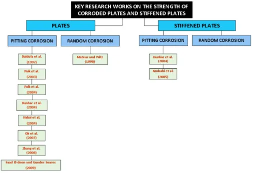
The problem of strength analysis of plates and stiffened plates incorporating different corrosion types has attracted the attention of some researchers. History tree of key research studies on the strength of corroded plates and stiffened plates is prepared and shown in the Fig. 3. Of course, there may be some other research works relevant to the subject of investigating the strength of corroded plates and stiffened plates. However, a set of research reports and investigations, that have been available to the authors, is reviewed herein.
Figure 3 History tree of key research studies on the strength of corroded plates and stiffened plates.
2.1 Pitted plates
Daidola et al. [4] proposed a mathematical model to estimate the residual thickness of pitted plates using the average and maximum values of pitting data or the number of pits and the depth of the deepest pit, and presented a method to assess the effect of thickness reduction due to pitting on local yielding and plate buckling based on the probabilistic approach. Fur-thermore, they developed a set of tools which can be used to assess the residual strength of pitted plates.
Paik et al. [14, 15] studied the ultimate strength characteristics of pitted plate elements under axial compressive loads and in-plane shear loads, and derived closed form formulae for predicting the ultimate strength of pitted plates using the strength reduction (knock-down) factor approach. They dealt with the case where the shape of corrosion pits is a cylinder.
post-ultimate responses of the corroded plates.
Nakai and his collaborators [10, 11] performed a series of nonlinear finite-element (FE) analyses with pitted plates subjected to in-plane compressive loads and bending moments in order to investigate their behaviours. They also established a method for prediction of ultimate strength of plate models with pitted corrosion.
Ok et al. [13] focused on assessing the effects of localised pitting corrosion which concen-trates at one or several possibly large area on the ultimate strength of unstiffened plates. They applied multi-variable regression method to derive new formulae to predict ultimate strength of unstiffened plates with localised corrosion. Their results indicated that the length, breadth and depth of pit corrosion have weakening effects on the ultimate strength of the plates while plate slenderness has only marginal effect on strength reduction. It was also revealed by them that transverse location of pit corrosion is an important factor determining the amount of strength reduction.
Zhang et al. [22] focused on the development of an assessing method for ultimate strength of ship hull plate with corrosion damnification. Pitting corrosion results in a quantity loss of the plate material as well as a significant degradation of the ultimate strength of the hull plate due to reducing of the effective thickness of the plate. Accordingly, the model for describing the correlations between the ultimate strength and the corroded volume loss of a corroded plate was proposed by them based on relative theory. Such model was then completed through numerical experiment by nonlinear finite element analyses for series of corroded plate models.
Later Saad Eldeen and Guedes Soares [16] investigated the collapse strength of pitted plates under in-plane compression. They performed some non-linear finite element analyses on the plates with different corrosion densities. Based on the obtained results, they could derive a formula in order to predict the ultimate strength reduction for the plates with pitting corrosion.
2.2 Pitted stiffened plates
Dunbar et al. [5], in some part of their research study, also investigated the collapse behaviour of stiffened plates under uni-axial compressive loads.
Besides, Amlashi and Moan [1] assessed the strength behaviour of stiffened plates under bi-axial compressive loading.
2.3 Randomly corroded plates
2.4 Randomly corroded stiffened plates
To the knowledge of authors, there is not any key research work investigating the strength and collapse behaviour of stiffened plates.
The main objective of the present paper is to examine how general corrosion affects ba-sic mechanical properties of plates and stiffened plates under compression and to explore the method of simulating behaviour of plated members with general corrosion by FE-analysis us-ing shell elements. This paper presents the results of an investigation into the post-bucklus-ing behaviour and ultimate strength of imperfect corroded steel plates and stiffened plates used in ship and other related marine structures. A series of elastic-plastic large deflection finite ele-ment analyses is performed on both-sides randomly corroded steel plates and stiffened plates. The effects of general corrosion are introduced into the finite element models using a ran-dom thickness surface model. The effects on buckling and ultimate strengths as a result of parametric variation of the corrosion age are evaluated.
3 DESCRIPTION OF STRUCTURAL MODELS 3.1 Extent of the models and their characteristics
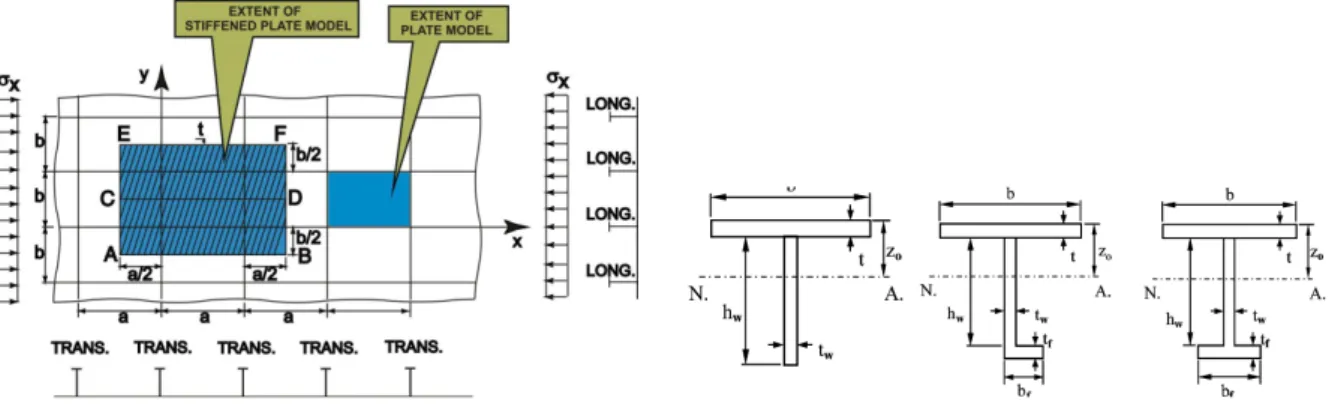
The plates in marine structures are of continuous nature. They are stiffened with longitudi-nal stiffeners and transverse frames. Longitudilongitudi-nal stiffeners and transverse frames divide the surface of the plates into isolated regions, Fig. 4(a). The filled region in Fig. 4(a) exhibits typically the extent of the plate models considered in the present investigation.
(a) Extent of the plate and stiffened plate models (b) Cross-sections of stiffeners in the stiffened plate model
Figure 4 Extent of the models and their characteristics.
A triple span- triple bay (TS-TB) model (region ABFE in Fig. 4 (a)) has been chosen for the analysis of buckling/plastic collapse behaviour of corroded stiffened plates with symmetri-cal/unsymmetrical stiffeners [20]. This is the most complete and precise extent of the stiffened plate models when analysing their behaviour [20].
types of models have been considered. In each type, three different shapes of stiffeners (Flat, Angle and Tee) have been attached to the isotropic plate, Fig. 4(b). The stiffeners of each type have the same moment of inertia. Types 1, 2 and 3 correspond respectively to weak, medium and heavy stiffeners.
In all analysed cases, local plate panels have a length of 2400 mm and a breadth of 800 mm.
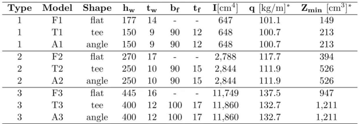
Table 1 Geometrical characteristics of the analysed models of stiffened plates.
Type Model Shape hw tw bf tf I[cm4] q [kg/m]∗ Zmin [cm3]∗
1 F1 flat 177 14 - - 647 101.1 149 1 T1 tee 150 9 90 12 648 100.7 213 1 A1 angle 150 9 90 12 648 100.7 213 2 F2 flat 270 17 - - 2,788 117.7 394 2 T2 tee 250 10 90 15 2,844 111.9 526 2 A2 angle 250 10 90 15 2,844 111.9 526 3 F3 flat 445 16 - - 11,749 137.5 947 3 T3 tee 400 12 100 17 11,860 132.7 1,211 3 A3 angle 400 12 100 17 11,860 132.7 1,211
∗ Z
minincludes width 800 mm of the plate having thickness of 13 mm
3.2 Loading and boundary conditions
As shown in Fig. 4(a), each region of the continuous plate is surrounded by longitudinal stiffeners and transverse frames. To consider the effects of longitudinal stiffeners and transverse frames in the model of isolated plates, proper boundary conditions are to be applied on it. Description of applied boundary conditions in the plate models is shown in Fig. 5(a).
On the other hand, the boundary conditions of the analysed stiffened plates are as follow:
• In the case of unsymmetrical stiffeners, periodically continuous conditions are imposed
at the same x-coordinate along the longitudinal edges (i.e. along AB and EF). These conditions are defined as below:
uAB=uEF wAB=wEF θx−AB=θx−EF θy−AB=θy−EF θz−AB=θz−EF
(1)
• In the case of symmetrical stiffeners, symmetry conditions are imposed at the same
(a) Loading and boundary conditions of the plate model
(b) Discretised finite element model of plate
(c) Discretised finite element models of plates with T-type and L-type stiffeners
Figure 5 Loading and boundary conditions.
• When the aspect ratio of the local plate panels is an even or odd number, then periodically
continuous conditions or symmetry conditions are imposed respectively at the same y-coordinate along the transverse edges in the model (i.e. along AE and BF).
• Although transverse frames are not modelled, the out-of-plane deformation of plate is
restrained along its junction line with the transverse frame.
• To consider the plate continuity, in-plane movement of the plate edges in their
perpen-dicular directions is assumed to be uniform.
Loading would be compressive along x-axis of the Fig. 4(a). The uniaxial compressive loading was applied by controlled edge displacement.
3.3 Finite Element code, adopted element and mesh density
buckling, and also to account for the continuity of the plate through the transverse frames. Furthermore, the mesh needs to be fine enough to recognize the initial imperfections to make sure that buckling occurs and to avoid unduly stiff behaviour. The buckling/plastic collapse behaviour and ultimate strength of models are hereby assessed using ANSYS [2], in which both material and geometric nonlinearities are taken into account. An APDL code was prepared inside ANSYS environment to facilitate parametric modelling and analysis using ANSYS [2].
Plates and stiffeners are modelled by SHELL181 elements with elastic-plastic large de-flection solution option. SHELL181 is suitable for analyzing thin to moderately-thick shell structures. It is a 4-node element with six degrees of freedom at each node: translations in the x, y, and z directions, and rotations about the x, y, and z-axes. SHELL181 is well-suited for linear, large rotation, and/or large strain nonlinear applications. Change in shell thickness is accounted for in nonlinear analyses. In order to obtain reasonable results a number of sen-sitivity analyses were carried out to find out the optimum mesh density and proper values of nonlinear analysis options. Samples of finite element descretisations are represented in Figs. 5(b) and 5(c).
3.4 Applied material properties
The material used in the models was of normal strength steel (abbreviated by NS steel) type. This type of steel has Young’s modulus of 21000 kgf/mm2
and Poisson’s ratio of 0.3. The yield strength of 24 kgf/mm2
is taken into account for NS steel.
It is evident that strain-hardening effect has some influence on the nonlinear behaviour of plates. The degree of such an influence is a function of many factors including plate slenderness. In this study, material behaviour for plate was modelled as a bi-linear elastic-plastic manner with strain-hardening rate of E/65, Fig. 6. This value of strain-hardening rate was obtained through a large number of elastic-plastic large deflection analyses made by Khedmati [8].
3.5 Initial deflections in plate and stiffener
The actual mode of the initial deflection of the plate is very complex, Fig. 7 [6, 7]. This complex mode can be expressed by a double sinusoidal series as:
w0= ∞
∑
m=1 ∞
∑
n=1
A0mnsin mπx a sin nπy b (2)
x
y
Figure 7 Real distribution of initial deflection or so-called thin-horse mode initial deflection [6, 7].
When compressive load acts in the direction of the longer side of the plate (x-direction), the deflection components in the direction of the shorter side of the plate (y-direction) decrease with the increase in load except the first term with one half-wave. In this case, only the first term (n=1) may play a dominant role, and the simpler form of initial deflection can be used for analysis as follows:
w0= ∞
∑
m=1
A0m1sin mπx
a sin πy
b (3)
Ueda and Yao [19] used only odd terms. Finally Yao et. al. [21] introduced even terms also in this mode, and the so-called “idealized thin-horse mode” took the following form:
w0= 11 ∑
m=1
A0m1sin mπx
a sin πy
b (4)
The coefficients of this mode are given in Table 2 [21] as functions of plate aspect ratio and its thickness. The coefficients are so scaled that the maximum magnitude of initial deflection,
w0 max, is to be as:
w0 max=0.05β 2
t (5)
Where β is the slenderness parameter of the plate and defined by:
β= b t
√σ Y
E (6)
Table 2 Coefficients of thin-horse mode initial deflection as a function of plate aspect ratio [21].
a/b A01/t A02/t A03/t A04/t A05/t A06/t 1<a/b<√2 1.1158 -0.0276 0.1377 0.0025 -0.0123 -0.0009
√
2<a/b<√6 1.1421 -0.0457 0.2284 0.0065 0.0326 -0.0022
√
6<a/b<√12 1.1458 -0.0616 0.3079 0.0229 0.1146 -0.0065
√
12<a/b<√20 1.1439 -0.0677 0.3385 0.0316 0.1579 -0.0149
√
20<a/b<√30 1.1271 -0.0697 0.3483 0.0375 0.1787 -0.0199
a/b A07/t A08/t A09/t A010/t A011/t 1<a/b<√2 -0.0043 0.0008 0.0039 -0.0002 -0.0011
√
2<a/b<√6 -0.0109 0.001 -0.0049 -0.0005 0.0027
√
6<a/b<√12 0.0327 0.000 0.000 -0.0015 -0.0074
√
12<a/b<√20 0.0743 0.0059 0.0293 -0.0012 0.0062
√
20<a/b<√30 0.0995 0.0107 0.0537 -0.0051 0.0256
The following initial imperfections were accounted for in analysing the stiffened plate mod-els in this study:
• Real distribution of initial deflection mode for the plate as explained by Eq. (4), as
represented by Fig. 8(a). This is a distinction point between this study and other related studies which have been previously done on the strength of corroded plates and stiffened plates. Mateus and Witz [9] assumed the following single-term expression for defining the initial deflection of the corroded plate based on simplified analyses made by Smith et al. [17]:
w0=0.1β 2
tsinπx
a sin πy
b (7)
(a) Initial deflection in the plate (b) Initial deflection in the stiffener (c) Angular distortion of the stiffener
Figure 8 Components of initial imperfections in the stiffened plate models.
• Initial deflection for the stiffener as expressed by Eq. (8) and represented by Fig. 8(b)
ws=(0.0025×a)sin πx
a (8)
• Angular distortion of the stiffener which is taken as (Fig. 8(c))
∅0hw=(0.0025×a)sin
πx
a (9)
The authors prepared a computer code in FORTRAN90 language in order to produce the initial imperfections expressed by Eqs. (4), (8) and (9) inside the models.
3.6 Random general corrosion modelling
A plate/stiffened plate subject to general corrosion has a random distribution of thickness over its area. The likelihood of these variations in thickness to form plastic hinges that may affect the buckling and post-buckling behaviour of a corroded plate/stiffened plate, and perhaps its ultimate strength, is something that cannot be discarded without further analysis [9].
The extent of general corrosion in marine structures is reflected in the results published by Ohyagi [12] based on the compilation of data gathered by Nippon Kaiji Kyokai (NKK) from corrosion surveys on ships. He gave the mean and minimum values of thickness measured at each inspection and also other statistical parameters of significance such as the standard deviation. According to the results of the NKK surveys, general cargo carriers are most affected by corrosion and the cargo holds are the most corroded spaces.
Ohyagi’s uniform thickness reduction general corrosion model has a mean linear trend for maximum corrosion rates. Besides, it is following a normal distribution for the probability of exceedance of corrosion rate and explained by [12]:
dw=0.34ny (10)
where ny is the number of years of exposure and dw is the uniform reduction in thickness in
millimeters after ny years of exposure. The standard deviation associated with the normal
distribution is 0.23mm, based on the studies of Ohyagi [12].
It may be reasonable to assume that the corroded surfaces of a plate with its random thickness variation is composed of an infinite summation of random coefficients associated with each of the elastic buckling modes of the plate. In numerical terms the general corrosion model describes the typical surfaces of a corroded plate as a random thickness variation, tp,
with an average value equal to the original thickness of plate, minus the corroded equivalent thickness reduction. The following expression was applied in the studies made by Mateus and Witz [9]
tp(x, y)=t−dw+ ∞
∑
i=1 ∞
∑
k=1
where Ai and Bk are the random coefficients associated with mode i in the x-direction and
the mode kin the y-direction, respectively and fi=sin(iπx/a),gk=sin(kπy/b).
Establishment of proper values for Ai and Bk in Eq. (8) is not so easy to the researchers.
That is why; instead of above-mentioned expression of double sinusoidal summation, a more practical way was adopted in this paper in order to generate randomly corroded surfaces for plates. A special purpose computer code was written in FORTRAN90 language. Generation of randomly corroded surfaces was achieved using the features of the GDIS function of FOR-TRAN90. The modified version of Eq. (11), which was developed and used in this research, can be expressed as:
tp(x, y)=t−dw+DRAN DM(0) (12)
There was one limitation in the generation process and it was standard deviation of the plate thicknesses at different nodes that was set to 0.23mm, as investigated by Ohyagi [12].
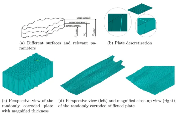
Different surfaces and relevant parameters corresponding to the case of a plate element with general corrosion are shown in Fig. 9(a). Definition of different layers in case of both-sides randomly distributed general corrosion is given in Fig. 9(b). Three different layers are considered through the thickness of each of the SHELL181 elements used for descretisation of the plate. The thickness of middle layer is equal to (t−dw), while the thicknesses of upper and
lower layers are adjusted by random values of r1,r2.
Finally, z-coordinate of upper and lower surfaces of both-sides randomly corroded plate can be defined as:
zLowSRF =w0− t−dw
2 −r1 , zU pSRF = w0+
t− dw
2 + r2 (13) where
tp=zU pSRF −zLowSRF =t−dw+r1+r2 (14)
Random values of r1and r2are produced by GDIS function.
The same procedure, as described above, was also applied to stiffener web and flange elements. Figures 9(c) and 9(d) exhibit respectively perspective views of typical both-sides randomly corroded plates and stiffened plates.
3.7 Validation
(a) Different surfaces and relevant pa-rameters
(b) Plate descretisation
(c) Perspective view of the randomly corroded plate with magnified thickness
(d) Perspective view (left) and magnified close-up view (right) of the randomly corroded stiffened plate
Figure 9 Finite element analysis modeling details for general corrosion.
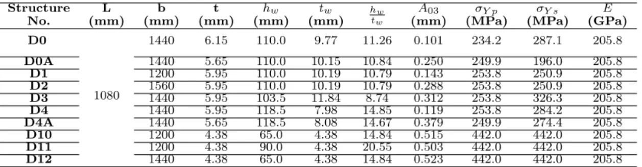
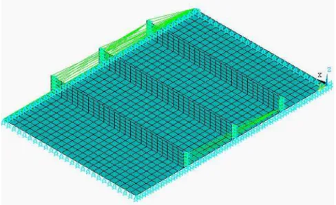
Fig. 11. To account for the effect of adjacent panels on the collapse behaviour of central panel, three-span models with two adjacent (dummy) stiffened panels and supported by two transverse frames were employed. The thickness of plate and stiffeners in two adjacent panels was 1.2-1.3 times that of plate and stiffeners in the central panel. Table 3, where L=1080mm is the span length of the plate with average plate thickness betweent=4.38mm tot=6.15mm, represents geometric and material properties for the Tanaka & Endo test structures. The boundaries of stiffened plates were continues simply supported and the in-plane axial compression load was applied longitudinally. The maximum measured initial deflections in the plate were ranging between 0.1-0.4 mm.
Figure 10 Stiffened plate model positioned in the Tanaka & Endo testing rig [18].
Figure 11 Tanaka & Endo test model [18].
Table 3 Geometric and material properties of Tanaka & Endo tests.
Structure L b t hw tw hw
tw
A03 σY p σY s E
No. (mm) (mm) (mm) (mm) (mm) (mm) (MPa) (MPa) (GPa)
D0
1080
1440 6.15 110.0 9.77 11.26 0.101 234.2 287.1 205.8
D0A 1440 5.65 110.0 10.15 10.84 0.250 249.9 196.0 205.8 D1 1200 5.95 110.0 10.19 10.79 0.143 253.8 250.9 205.8 D2 1560 5.95 110.0 10.19 10.79 0.288 253.8 250.9 205.8 D3 1440 5.95 103.5 11.84 8.74 0.312 253.8 326.3 205.8 D4 1440 5.95 118.5 7.98 14.85 0.119 253.8 284.2 205.8 D4A 1440 5.65 118.5 8.08 14.67 0.379 249.9 274.4 205.8 D10 1200 4.38 65.0 4.38 14.84 0.515 442.0 442.0 205.8 D11 1200 4.38 90.0 4.38 20.55 0.503 442.0 442.0 205.8 D12 1440 4.38 65.0 4.38 14.84 0.523 442.0 442.0 205.8
σU lt=Pu/(Ap+As) (15)
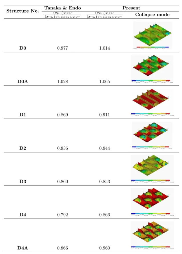
A summary of the results obtained through the finite element simulation of the tests carried out by Tanaka & Endo is given in Table 4. Also, in these tables, the obtained collapse modes from FEM analyses are shown. Comparison of the results show that in general good agreement exists among the FEM results with those obtained from the tests.
Table 4 Summary of results for some of Tanaka & Endo tests. Structure No. Tanaka & Endo(σU lt)F EM Present
(σU lt)EXP ERIM EN T
(σU lt)F EM
(σU lt)EXP ERIM EN T Collapse mode
D0 0.977 1.014
D0A 1.028 1.065
D1 0.869 0.911
D2 0.936 0.944
D3 0.860 0.853
D4 0.792 0.866
Interactive buckling in both plate and stiffeners can be observed in other models, where the level of plastic deformations, in the plate varies among them. The values of the ultimate strength predicted by FEM in this work are in better consistency as compared with those obtained by Tanaka & Endo [18]. The reason may be due to the fact that in such cases, the initial deflection of the test specimens was simulated in FEM with a better accuracy.
Figure 12 Finite element model of Tanaka & Endo test specimens.
4 INVESTIGATED PARAMETRIC MODELS 4.1 Plate models
In order to study the effects of random thickness variation on the response of axially loaded plates, different cases were considered. The cases included in the study are briefly explained in the following
• Corroded plates with AR=2,t=10-20 mm andS=0.23 made of NS steel
• Corroded plates with AR=3,t=10-20 mm andS=0.23 made of NS steel
4.2 Stiffened plate models
Besides, in order to study the effects of random thickness variation on the response of axially loaded stiffened plates, the following cases were generated and considered
• Plate aspect ratio: AR = 3
• Stiffener type, shape and size: F1, F2,F3,T1,T2,T3,L1,L2,L3
• Mean corrosion depth: µ= 2mm
• Standard deviation of random thickness variations: S = 0.2, 0.4 mm
• Material: NS steel
5 RESULTS AND DISCUSSIONS 5.1 Plate models
For each of above cases, different models were created changing the age of the plate. The ages considered for the models were 5, 10, 15 and 20 years of exposure to the sea water. The corroded surfaces of the models were different in these cases. All of the plate models were analysed under longitudinal in-plane compression. Average stress-average strain relationships for the models are shown respectively in the Figs. 13 to 18. The maximum magnitude of thin-horse mode initial deflection for the corroded models is calculated using the Eq. (5) for the original thickness. Also, Von Mises stress distributions are shown for a selection of the cases representing thin and thick plates in Tables 5, 6, 7 and 8. On the other hand, Tables 9, 10, 11 and 12 give a summary of results regarding degradation of the buckling/ultimate strength as results of corrosion of the plate.
The average stress-average strain relationships of the plate models in un-corroded condition are shown in the Figs 13 to 16 for selected thin and thick plates.
Figures 13 to 18 in addition to the results summarised in Tables 5 to 12 reveal the following main characteristics for the buckling/ultimate strengths and behaviours of the corroded plate models.
• Age or sea exposure life of the plate models affects mainly their post-buckling-strength
regimes and degrades their buckling/ultimate strength.
• Average stress-average strain relationships of the thin plates at lower exposure times
and also those of the thick plates at upper exposure times show snap-back behaviours of the plate (Figs. 13, 17, 18 and also table 5). This is mainly due to the very thin plate of both-sides randomly corroded plate. The ultimate strength or collapse mode of the plate of aspect ratio equal to 2 with the original un-corroded thickness of 14 mm exhibit creation of three buckling half-waves as a result of snap-back behaviours described above.
• Thin plates at all ages and also thick plates at upper exposure time show that they
un-dergo elastic buckling with distinct distance between the buckling and ultimate strength levels, Figs. 13 to 18.
• Figures 13, 15 and 17 reveals the fact that for the thin/thick plates having the aspect
Table 5 Deformation mode and spread of plasticity for the plate of dimensions 1600×800×14 mm (AR=2)
with 5-20 years exposure (magnification factor for deformation mode: 10).
Case Ultimate strength level Final step
Uncorroded
t=14 mm
5-year
t=13.17 mm
10-year
t=11.73 mm
15-year
t=9.94 mm
20-year
t=8.18 mm
thin/thick plate is 3, the ultimate strain remains almost unchanged while the ultimate strength decreases as a direct function of exposure time, Figs. 14, 16 and 18. Thus, one of the main factors influencing the ultimate strength of the corroded steel plates would be their aspect ratio.
• The post-ultimate-strength regimes of the corroded thin/thick plate show a uniform
reduction in the reserve strength of the plate as its exposure time increases, Figs. 13 to 16.
Table 6 Deformation mode and spread of plasticity for the plate of dimensions 2400×800×14 mm (AR=3)
with 5-20 years exposure (magnification factor for deformation mode: 10).
Case Ultimate strength level Final step
Uncorroded
t=14 mm
5-year
t=13.3 mm
10-year
t=11.75 mm
15-year
t=10.04 mm
20-year
t=8.23 mm
almost regular half-waves are generated inside the plate extent in longitudinal direction at the ultimate strength level. Besides, post-ultimate-strength mode shapes show the local accumulation of deflection in some regions of the plate model in addition to the unloading the rest of plate area. The place of local deflection accumulation is not fixed and in other words changed from case to case.
• Tables 9 to 12 represent the degradation percentages of the buckling and ultimate
strengths of the corroded plates. The difference values are defined as follows
⎧ ⎪ ⎪ ⎪ ⎪ ⎪ ⎪ ⎨ ⎪ ⎪ ⎪ ⎪ ⎪ ⎪ ⎩
(∆σ)Cr= (σCr)U ncorroded−(σCr)Corroded (σCr)U ncorroded
×100
(∆σ)U lt= (σU lt)U ncorroded−(σU lt)Corroded (σU lt)U ncorroded
×100
Table 7 Deformation mode and spread of plasticity for the plate of dimensions 1600×800×18 mm (AR=2)
with 5-20 years exposure (magnification factor for deformation mode: 10).
Case Ultimate strength level Final step
Uncorroded
t=18 mm
5-year
t=17.47 mm
10-year
t=15.50 mm
15-year
t=13.79 mm
20-year
t=12.43 mm
Table 8 Deformation mode and spread of plasticity for the plate of dimensions 2400×800×18 mm (AR=3)
with 5-20 years exposure (magnification factor for deformation mode: 10).
Case Ultimate strength level Final step
Uncorroded
t=18 mm
5-year
t=17.47 mm
10-year
t=15.50 mm
15-year
t=13.79 mm
20-year
Table 9 Comparison of results for plate 1600×800×14 mm with 0-20 years of exposure.
Case Buckling StrengthσCr Ultimate Strength
σY p (∆σ)Cr
σU lt
σY p (∆σ)U lt
uncorroded 0.643 0 0.772 0 5-year exposure 0.596 7.39 0.724 6.21 10-year exposure 0.471 26.68 0.601 22.15 15-year exposure 0.280 56.45 0.535 30.67 20-year exposure 0.204 68.20 0.476 38.39
Table 10 Comparison of results for plate 2400×800×14 mm with 0-20 years of exposure.
Case Buckling StrengthσCr Ultimate Strength
σY p (∆σ)Cr
σU lt
σY p (∆σ)U lt
uncorroded 0.661 0 0.750 0 5-year exposure 0.602 8.99 0.701 6.46 10-year exposure 0.472 28.67 0.634 15.49 15-year exposure 0.348 47.38 0.575 23.27 20-year exposure 0.253 61.67 0.531 29.22
Table 11 Comparison of results for plate 1600×800×18 mm with 0-20 years of exposure.
Case Buckling StrengthσCr Ultimate Strength
σY p (∆σ)Cr
σU lt
σY p (∆σ)U lt
uncorroded 0.889 0 0.931 0 5-year exposure 0.8229 7.50 0.885 4.91 10-year exposure 0.7769 12.66 0.841 9.62 15-year exposure 0.617 30.60 0.760 18.34 20-year exposure 0.475 46.50 0.632 32.13
Table 12 Comparison of results for plate 2400×800×18 mm with 0-20 years of exposure.
Case Buckling StrengthσCr Ultimate Strength
σY p (∆σ)Cr
σU lt
σY p (∆σ)U lt
Figure 13 Comparison of average stress-average strain relationships for a plate with random distribution of corrosion (a=1600mm,b=800
mm,t=14mm,S=0.23).
Figure 14 Comparison of average stress-average strain relationships for a plate with random distribution of corrosion (a=2400mm,b=800
mm,t=14mm,S=0.23).
Figure 15 Comparison of average stress-average strain relationships for a plate with random distribution of corrosion (a=1600mm,b=800
mm,t=18mm,S=0.23).
Figure 16 Comparison of average stress-average strain relationships for a plate with random distribution of corrosion (a=2400mm,b=800
(a) 5-year exposure (b) 10-year exposure
(c) 15-year exposure (d) 20-year exposure
(a) 5-year exposure (b) 10-year exposure
(c) 15-year exposure (d) 20-year exposure
5.2 Stiffened plate models
For each of the above-mentioned cases, 50 models were created changing the random thickness variation parameters. The corroded surfaces of the models were different in these cases. Gaus-sian distribution for random thickness variation was considered in all cases and corresponding models. All of the stiffened plate models were analysed under longitudinal in-plane compres-sion. Average stress-average strain relationships for the stiffened plate models with flat-bar, tee-bar and angle-bar stiffeners are respectively shown in Fig. 19, Fig. 20 and Fig. 21. Also, Von Mises stress distributions and deflection modes at ultimate strength level and final step of calculations are shown for a selection of the cases in Tables 13, 14 and 15.
(a) F1 model (b) F2 model (c) F3 model
Figure 19 Comparison of average stress-average strain relationships for corroded stiffened plates withAR=3,
t=13mm, stiffener typeF, mean corrosion depth = 2mm andS=0.2mm made of NS steel.
(a) T1 model (b) T2 model (c) T3 model
(a) L1 model (b) L2 model (c) L3 model
Figure 21 Comparison of average stress-average strain relationships for corroded stiffened plates withAR=3, t=13mm, stiffener typeL, mean corrosion depth = 2mm andS=0.2mm made of NS steel.
The maximum magnitude of thin-horse mode initial deflection for the plate part in corroded models is calculated using Eq. (5) based on the original thickness of the plate. The average stress-average strain relationships of the stiffened plate models in un-corroded condition as well as in the condition of having uniform thickness reduction are shown in Figs. 19 to 21. The stiffened plate in the condition of uniform corrosion or uniform thickness reduction has a reduction equal to the mean corrosion depth from original un-corroded thickness for its plate and stiffener parts.
Figures 19 to 21 in addition to the results summarised in Tables 13 to 15 reveal the follow-ing main characteristics for the bucklfollow-ing/ultimate strengths and behaviours of the corroded stiffened plate models
• Random thickness variations in the stiffened plate model surfaces mainly affect their
post-ultimate-strength regimes while their pre-ultimate-strength behaviours are almost unchanged. When the average stress-average strain relationships of 50 models analysed in any case are drawn, their post-ultimate-strength regions create a band. Such a band in post-ultimate-strength regions has a lower limit and an upper limit.
• The curve of average stress-average strain for the condition of uniformly corroded
Table 13 A selection of stress distributions and deflection modes for corroded stiffened plate model F3 at ultimate strength level and final step of calculations (magnification factor for deflection mode: 10). Plate 2400 × 800 × 13, F3 model, 2mm Corrosion, S=0.2 mm, NS steel
Case Ultimate strength step σave
σY Final Step
ε εY =3
σave
σY
No
Corrosion 0.759 0.462
Uniform
Corrosion 0.678 0.421
Random Upper
Band
0.678 0.423
Random Lower
Band
0.675 0.358
• The trends of the curves in the post-ultimate-strength regions are not always entirely
sim-ilar to each other. In some cases, local descending or ascending behaviours are observed on the post-ultimate-strength regions of the average stress-average strain curves.
• The mode shapes and Von Mises stress contours shown in Tables 13 to 15 reveal that
almost regular half-waves are generated inside the stiffened plate components in longi-tudinal direction at the ultimate strength level. Besides, post-ultimate-strength mode shapes show that local accumulation of deflection in some regions of the model in ad-dition to the unloading the rest of model are occurred. The place of local deflection accumulation is not fixed and, in other words, changes from case to case.
• In all cases, a remarkable drop in the value of ultimate strength and buckling strength
Table 14 A selection of stress distributions and deflection modes for corroded stiffened plate model T3 at ultimate strength level and final step of calculations (magnification factor for deflection mode: 10). Plate 2400 × 800 × 13, T3 model, 2mm Corrosion, S=0.2 mm, NS steel
Case Ultimate strength step σave
σY Final Step
ε εY =3
σave
σY
No
Corrosion 0.841 0.418
Uniform
Corrosion 0.764 0.376
Random Upper
Band
0.766 0.404
Random Lower
Band
0.762 0.377
suffer from random general corrosion.
6 CONCLUSIONS
Table 15 A selection of stress distributions and deflection modes for corroded stiffened plate model L3 at ultimate strength level and final step of calculations (magnification factor for deflection mode: 10). Plate 2400 × 800 × 13, L3 model, 2mm Corrosion, S=0.2 mm, NS steel
Case Ultimate strength step σave
σY Final Step
ε εY =3
σave
σY
No
Corrosion 0.871 0.444
Uniform
Corrosion 0.795 0.401
Random Upper
Band
0.791 0.495
Random Lower
Band
0.790 0.398
outcomes can be summarised as follows:
• Aspect ratio and thickness (slenderness) of the plate have different effects on the strength
characteristics of the corroded plate.
• Age or sea exposure time of the plate models affects mainly their post-buckling-strength
regimes and degrades their buckling/ultimate strength.
• Snap-back behaviours are seen in the average stress-average strain relationships of the
corroded plate elements, especially when their slenderness parameter falls to the range of thin plates.
• Reduction in the buckling strength of both-sides randomly corroded steel plates is
to the ultimate strength at a specific exposure time may be sometimes about 2.
• Random thickness variations in the stiffened plate model surfaces mainly affect their
post-ultimate-strength regimes while their pre-ultimate-strength behaviours are almost unchanged.
• The condition of uniformly corroded stiffened plate almost in all cases exhibits an
inter-mediate condition for randomly corroded stiffened plates.
• A remarkable drop in the value of ultimate strength and buckling strength of the stiffened
plate models, as a result of random general corrosion is seen.
References
[1] H.K.K. Amlashi and T. Moan. On the strength assessment of pitted stiffened plates under biaxial compression loading. In24th international conference on offshore mechanics and arctic engineering, Halkidiki, Greece, 2005.
[2] ANSYS Inc. ANSYS 11.0 Reference Manual, 2008.
[3] ASM International Corrosion. ASM Handbook, 2001. Vol. 13.
[4] J.C. Daidola, J. Parente, I.R. Orisamolu, and K.T. Ma. Residual strength assessment of pitted plate panels. Technical Report SSC-394, Ship Structure Committee, 1997.
[5] T.E. Dunbar et al. A computational investigation of the effects of localized corrosion on plates and stiffened panels. Mar Struct, 17(5):385–402, 2004.
[6] M. Fujikubo, S. Harada, T. Yao, M.R. Khedmati, and D. Yanagihara. Estimation of ultimate strength of continuous stiffened panel under combined transverse thrust and lateral pressure, Part 2: Continuous stiffened panel. Marine Structures, 18:411–417, 2005.
[7] M. Fujikubo, T. Yao, M.R. Khedmati, S. Harada, and D. Yanagihara. Estimation of ultimate strength of continuous stiffened panel under combined transverse thrust and lateral pressure, Part 1: Continuous plate. Marine Structures, 18:383–410, 2005.
[8] M.R. Khedmati. Ultimate strength of ship structural members and systems considering local pressure loads.Graduate School of Engineering, Hiroshima University, 2000. Dr. Eng. Thesis.
[9] A.F. Mateus and J.A. Witz. On the buckling and post-buckling of corroded steel plates. Royal Institution of Naval Architects, Transactions Part C, 140, 1998.
[10] T. Nakai, H. Matsushita, and N. Yamamoto. Effect of pitting corrosion on local strength of hold frames of bulk carriers (1st report). Mar Struct, 17:403–432, 2004.
[11] T. Nakai, H. Matsushita, and N. Yamamoto. Effect of pitting corrosion on local strength of hold frames of bulk carriers (2nd report) Lateral-distortional buckling and local face buckling. Mar Struct, 17:612–641, 2004.
[12] M. Ohyagi. Statistical survey on wear of ship’s structural members. NK Technical Bulletin, Tokyo, 1987.
[13] D. Ok, Y. Pu, and A. Incecik. Computation of ultimate strength of locally corroded unstiffened plates under uniaxial compression.Mar Struct, 20:100–114, 2007.
[14] J.K. Paik, J.M. Lee, and M.J. Ko. Ultimate compressive strength of plate elements with pit corrosion wastage. J Eng Mar Environ, 217(M4):185–200, 2003.
[15] J.K. Paik, J.M. Lee, and M.J. Ko. Ultimate shear strength of plate elements with pit corrosion wastage. Thin-Wall Struct, 42:1161–1176, 2004.
[16] S. Saad Eldeen and C. Guedes Soares. Effect of pitting corrosion on the collapse strength of rectangular plates under axial compression. InProceedings of Analysis and Design of Marine Structures, pages 231–236, Potugal, 2009.
[18] Y. Tanaka and H. Endo. Ultimate strength of stiffened plates with their stiffeners locally buckled in compression. Journal of the Society of Naval Architects of Japan, 164, 1988. (in Japanese).
[19] Y. Ueda and T. Yao. The influence of complex initial deflection on the behaviour and ultimate strength of rectangular plates in compression. J. of Const. Steel Research, 5:265–302, 1985.
[20] T. Yao, M. Fujikubo, D. Yanagihara, and M. Irisawa. Consideration on fem modelling for buckling/plastic collapse analysis of stiffened plates.Trans. of the West-Japan Soc. Naval Arch., 85:121–128, 1998. (in Japanese).
[21] T. Yao, P.I. Nikolov, and Y. Miyagawa. Influence of welding imperfections on stiffness of rectangular plates under thrust. In K. Karlsson, L.E. Lindgren, and M. Jonsson, editors,Proc. of IUTAM Sump. on Mechanical Effects of Welding, pages 261–268. Springer-Verlag, 1992.
![Figure 1 Pitted web plate of the hold frame of a bulk carrier [10].](https://thumb-eu.123doks.com/thumbv2/123dok_br/18884364.423470/3.892.139.705.309.505/figure-pitted-web-plate-hold-frame-bulk-carrier.webp)
![Figure 7 Real distribution of initial deflection or so-called thin-horse mode initial deflection [6, 7].](https://thumb-eu.123doks.com/thumbv2/123dok_br/18884364.423470/10.892.274.678.211.449/figure-real-distribution-initial-deflection-called-initial-deflection.webp)
![Table 2 Coefficients of thin-horse mode initial deflection as a function of plate aspect ratio [21].](https://thumb-eu.123doks.com/thumbv2/123dok_br/18884364.423470/11.892.200.645.148.340/table-coefficients-horse-initial-deflection-function-plate-aspect.webp)